Simulink and the DSP Blockset (DSP Blockset)

DSP Blockset

Discrete-Time Signals

In theory, a discrete-time signal is defined by a sequence of values corresponding to particular instants in time. The time instants where the signal is defined are called the signal's sample times; traditionally, a discrete signal is considered to be undefined at points in time between these instants. For a periodically sampled signal, the equal interval between any pair of sample times is the signal's sample period, T_s. The sample rate, F_s, is the reciprocal of the sample period, or 1/T_s.

For example, the 7.5-second triangle wave segment below has a sample period of 0.5 sec, and sample times of 0.0, 0.5, 1.0, 1.5, ...,7.5. The sample frequency of the sequence is therefore 1/0.5, or 2 Hz.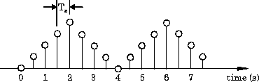

Time and Frequency Terminology

A number of different terms are used in this book to describe the characteristics of discrete-time signals found in Simulink models. These terms, which are listed in the table below, are frequently used in Chapter 4, "DSP Block Reference," to describe the way that various blocks operate on sample-based and frame-based signals. For additional information on frame-based processing, see "Understanding Samples and Frames" in this chapter.


Term	Symbol	Units	Notes
Sample period	T_s, T_si, T_so, t	Seconds	The time interval between consecutive samples in a sequence, as the input to a block (T_si) or the output from a block (T_so). T_si = T_fi if the input is sample based. T_so = T_fo if the output is sample-based.
Frame period, Input period, Output period	T_f, T_fi, T_fo	Seconds	The time interval between consecutive frames in a sequence, as the input to a block (T_fi) or the output from a block (T_fo). T_fi = T_si if the input is sample based. T_fo = T_so if the output is sample based.
Signal period	T	Seconds	The time elapsed during a single repetition of a periodic signal.
Sample rate, Sample frequency	F_s	Hz (samples per second)	The number of samples per unit time, F_s = 1/T_s.
Frequency	f	Hz (cycles per second)	The number of repetitions per unit time of a periodic signal, f = 1/T.
Normalized frequency	f_n	Two cycles per sample	Frequency of a periodic signal normalized to the Nyquist frequency, f_n = _n/ = 2f/F_s.
Angular frequency		Rads per sec	Frequency of a periodic signal in angular units, = 2f.
Digital (normalized angular) frequency	_n	Rads per sample	Frequency of a periodic signal normalized to the sample frequency, _n = /F_s = f_n

Discrete-Time Signals in Simulink

Simulink allows you to select from among several different simulation solver algorithms through the Solver options panel in the Simulation Parameters dialog box.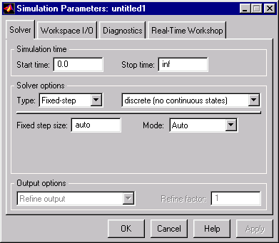

Recommended Simulation Settings for DSP. The recommended Solver options settings for DSP simulations are:

Type = Fixed-step discrete
Fixed step size = auto
Mode = Auto

With these settings, discrete signals in Simulink most accurately model the prototypical discrete signal described in the previous section. In particular, when these settings are in effect, discrete signals are undefined between sample times. Simulink generates an error when operations attempt to reference the undefined region of a signal, for example, when signals with different sample rates are added.

To perform cross-rate operations like the addition of two signals with different sample rates, you must explicitly convert the two signals to a common sample rate. There are several blocks provided for precisely this purpose in the Signal Operations and Multirate Filtering libraries. See "Rate Conversion," later in this section, for more information. By requiring explicit rate conversions for cross-rate operations, Simulink helps you to identify sample rate conversion issues early in the design process.

You can automatically set the above solver options for all new models by running the dspstartup M-file. See "Configuring Simulink for DSP Systems" earlier in this chapter for more information.

Note
In the block dialog boxes, the term sample time is often used to refer to the sample period, T_s. An example is the Sample time parameter in the Signal From Workspace block, which specifies the imported signal's sample period.

Other Simulation Settings. It is worthwhile to know how the other solver options available in Simulink affect discrete signals. In particular, you should be aware of the properties of discrete signals under the following options:

Variable-step (Simulink's default solver)
Fixed-step, Mode = SingleTasking

In both cases, discrete-time signals differ from the prototype described earlier by remaining defined between sample times. For example, the representation of the discrete-time triangle wave looks like this:

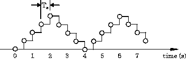
Because Simulink blocks typically apply a zero-order hold (ZOH) to outputs, the value of the signal between two adjacent sample times is the value at the earlier sample time. As an example, the signal's value at t=3.112 seconds is the same as the signal's value at t=3 seconds. In these two modes, a signal's sample times are the instants where the signal is allowed to change values, rather than where the signal is defined. Between the sample times, the signal is frozen at its last value.

As a result, in the Variable step and Fixed-step SingleTasking modes, Simulink permits cross-rate operations such as the addition of two signals of different rates. The next section explains how this works.

More About Variable-Step and Fixed-Step SingleTasking Modes. Because in these modes a discrete-time signal is defined between sample times, if you sample the signal with a rate or phase that is distinct from the signal's own rate and phase, you still measure meaningful values.

Consider the model below, which sums two signals having different sample periods. The fast signal (T_s=1) has sample times 1, 2, 3, ..., and the slow signal (T_s=2) has sample times 1, 3, 5, ....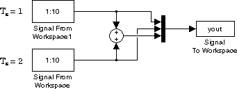

The output, yout, is a matrix containing the fast signal (T_s=1) in the first column, the slow signal (T_s=2) in the second column, and the sum of the two in the third column.

yout =
     1     1     2
     2     1     3
     3     2     5
     4     2     6
     5     3     8
     6     3     9
     7     4    11
     8     4    12
     9     5    14
    10     5    15

As expected, the slow signal (second column) changes once every two seconds, half as often as the fast signal. Nevertheless, it has a defined value at every moment in-between because of the zero-order hold that the Signal From Workspace block applies to the output. (Simulink implicitly auto-promotes the rate of the slower signal to match the rate of the faster signal before the addition operation is performed.)

In general, for Variable-step and Fixed-step SingleTasking modes, when you measure the value of a discrete signal in-between sample times, you are observing the value of the signal at the most recent sample time.

Sample Time Offsets. Simulink offers the ability to shift a signal's sample times by an arbitrary value, which is equivalent to shifting the signal's phase by a fractional sample period. However, sample-time offsets are rarely used in DSP systems, and blocks from the DSP Blockset do not support them.

[ Previous | Help Desk | Next ]