Stream Line Plots of Vector Data
MATLAB includes a vector data set called wind that represents air currents over North America. This example uses a combination of techniques:
Determine the Range of the Coordinates
Load the data and determine minimum and maximum values to locate the slice planes and contour plots (load, min, max).
load wind
xmin = min(x(:));
xmax = max(x(:));
ymax = max(y(:));
zmin = min(z(:));
Add Slice Planes for Visual Context
Calculate the magnitude of the vector field (which represents wind speed) to generate scalar data for the slice command. Create slice planes along the x-axis at xmin, 100, and xmax, along the y-axis at ymax, and along the z-axis at zmin. Specify interpolated face coloring so the slice coloring indicates wind speed, and do not draw edges (sqrt, slice, FaceColor, EdgeColor).
wind_speed = sqrt(u.^2 + v.^2 + w.^2);
hsurfaces = slice(x,y,z,wind_speed,[xmin,100,xmax],ymax,zmin);
set(hsurfaces,'FaceColor','interp','EdgeColor','none')
Add Contour Lines to the Slice Planes
Draw light gray contour lines on the slice planes to help quantify the color mapping (contourslice, EdgeColor, LineWidth).
hcont = ...
contourslice(x,y,z,wind_speed,[xmin,100,xmax],ymax,zmin);
set(hcont,'EdgeColor',[.7,.7,.7],'LineWidth',.5)
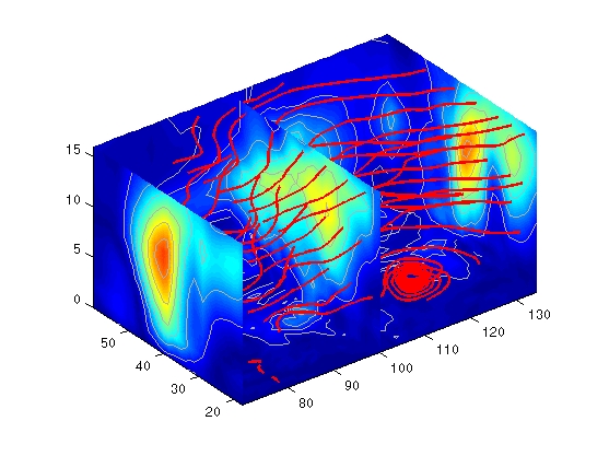
Define the Starting Points for the Stream Lines
In this example, all stream lines start at an x-axis value of 80 and span the range 20 to 50 in the y direction and 0 to 15 in the z direction. Save the handles of the stream lines and set the line width and color (meshgrid, streamline, LineWidth, Color).
[sx,sy,sz] = meshgrid(80,20:10:50,0:5:15);
hlines = streamline(x,y,z,y,v,w,sx,sy,sz);
set(hlines,'LineWidth',2,'Color','r')
Define the View
Set up the view, expanding the z-axis to make it easier to read the graph (view, daspect, axis).
view(3)
daspect([2,2,1])
axis tight
See coneplot for an example of the same data plotted with cones.
[ Previous | Help Desk | Next ]