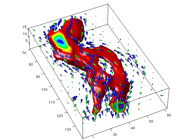
Volume Visualization Techniques (Using MATLAB Graphics)

Using MATLAB Graphics

Vector Data Displayed with Cone Plots

This example plots the velocity vector cones for the wind data. The graph produced employs a number of visualization techniques:

An isosurface is used to provide visual context for the cone plots and to provide means to select a specific data value for a set of cones.
Lighting enables the shape of the isosurface to be clearly visible.
The use of perspective projection, camera positioning, and view angle adjustments compose the final view.

Create an Isosurface

Displaying an isosurface within the rectangular space of the data provides a visual context for the cone plot. Creating the isosurface requires a number of steps:

Calculate the magnitude of the vector field, which represents the speed of the wind.
Use isosurface and patch to draw an isosurface illustrating where in the rectangular space the wind speed is equal to a particular value. Regions inside the isosurface have higher wind speeds, regions outside the isosurface have lower wind speeds.
Use isonormals to compute vertex normals of the isosurface from the volume data rather than calculate the normals from the triangles used to render the isosurface. These normals generally produce more accurate results.

Set visual properties of the isosurface, making it red and without edges drawn (FaceColor, EdgeColor).

load wind
wind_speed = sqrt(u.^2 + v.^2 + w.^2);
hiso = patch(isosurface(x,y,z,wind_speed,40));
isonormals(x,y,z,wind_speed,hiso)
set(hiso,'FaceColor','red','EdgeColor','none');

Adding Isocaps to the Isosurface

Isocaps are similar to slice planes in that they show a cross section of the volume. They are designed to be the end caps of isosurfaces. Using interpolated face color on an isocap causes a mapping of data value to color in the current colormap. To create isocaps for the isosurface, define them at the same isovalue (isocaps, patch, colormap).

hcap = patch(isocaps(x,y,z,wind_speed,40),...
    'FaceColor','interp',...
    'EdgeColor','none');
colormap hsv

Create First Set of Cones

Use daspect to set the data aspect ratio of the axes before calling coneplot so MATLAB can determine the proper size of the cones.
Determine the points at which to place cones by calculating another isosurface that has a smaller isovalue (so the cones display outside the first isosurface) and use reducepatch to reduce number of faces and vertices (so there are not too many cones on the graph).

Draw the cones and set the face color to blue and the edge color to none.

daspect([1,1,1]);
[f verts] = reducepatch(isosurface(x,y,z,wind_speed,30),0.07); 
h1 = coneplot(x,y,z,u,v,w,verts(:,1),verts(:,2),verts(:,3),3);
set(h1,'FaceColor','blue','EdgeColor','none');

Create Second Set of Cones

Create a second set of points at values that span the data range (linspace, meshgrid).

Draw a second set of cones and set the face color to green and the edge color to none.

xrange = linspace(min(x(:)),max(x(:)),10);
yrange = linspace(min(y(:)),max(y(:)),10);
zrange = 3:4:15;
[cx,cy,cz] = meshgrid(xrange,yrange,zrange);
h2 = coneplot(x,y,z,u,v,w,cx,cy,cz,2);
set(h2,'FaceColor','green','EdgeColor','none');

Define the View

Use the axis command to set the axis limits equal to the minimum and maximum values of the data and enclose the graph in a box to improve the sense of a volume (box).
Set the projection type to perspective to create a more natural view of the volume. Set the view point and zoom in to make the scene larger (camproj, camzoom, view).

Add Lighting

Add a light source and use Phong lighting for the smoothest lighting of the isosurface. Increase the strength of the background lighting on the isocaps to make them brighter (camlight, lighting, AmbientStrength).

camlight(-45,45)
lighting phong
set(hcap,'AmbientStrength',.6)

[ Previous | Help Desk | Next ]