linfun (Using Simulink)

Extract the linear state-space model of a system around an operating point.

Syntax

[A,B,C,D] = linfun('sys')
[A,B,C,D] = linfun('sys', x, u)
[A,B,C,D] = linfun('sys', x, u, pert)
[A,B,C,D] = linfun('sys', x, u, pert, xpert, upert)

Arguments


`linfun`	`linmod`, `dlinmod`, or `linmod2`.
`sys`	The name of the Simulink system from which the linear model is to be extracted.
`x` and `u`	The state and the input vectors. If specified, they set the operating point at which the linear model is to be extracted.
`pert`	Optional scalar perturbation factor used for both `x` and `u`. If not specified, a default value of 1e-5 is used.
`xpert` and `upert`	Optional vectors that explicitly set perturbation levels for individual states and inputs. If specified, the `pert` argument is ignored. The `i`th state `x` is perturbed to `x(i) + xpert(i)` The `j`th input `u` is perturbed to `u(j) + upert(j)`

Description

linmod obtains linear models from systems of ordinary differential equations described as Simulink models. linmod returns the linear model in state-space form, A, B, C, D, which describes the linearized input-output relationship:

Inputs and outputs are denoted in Simulink block diagrams using Inport and Outport blocks.

[A,B,C,D] = linmod('sys') obtains the linearized model of sys around an operating point with the state variables x and the input u set to zero.

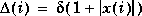
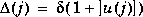
linmod perturbs the states around the operating point to determine the rate of change in the state derivatives and outputs (Jacobians). This result is used to calculate the state-space matrices. Each state x(i) is perturbed to

where

Likewise the jth input is perturbed to

where

Discrete-Time System Linearization

The function dlinmod can linearize discrete, multirate, and hybrid continuous and discrete systems at any given sampling time. Use the same calling syntax for dlinmod as for linmod, but insert the sample time at which to perform the linearization as the second argument. For example

[Ad,Bd,Cd,Dd] = dlinmod('sys', Ts, x, u);

produces a discrete state-space model at the sampling time Ts and the operating point given by the state vector x and input vector u. To obtain a continuous model approximation of a discrete system, set Ts to 0.

For systems composed of linear, multirate, discrete, and continuous blocks, dlinmod produces linear models having identical frequency and time responses (for constant inputs) at the converted sampling time Ts, provided that:

Ts is an integer multiple of all the sampling times in the system.
Ts is not less than the slowest sample time in the system.
The system is stable.

It is possible for valid linear models to be obtained when these conditions are not met.

Computing the eigenvalues of the linearized matrix Ad provides an indication of the stability of the system. The system is stable if Ts>0 and the eigenvalues are within the unit circle, as determined by this statement:

all(abs(eig(Ad))) < 1

Likewise, the system is stable if Ts = 0 and the eigenvalues are in the left half plane, as determined by this statement:

all(real(eig(Ad))) < 0

When the system is unstable and the sample time is not an integer multiple of the other sampling times, dlinmod produces Ad and Bd matrices, which may be complex. The eigenvalues of the Ad matrix in this case still, however, provide a good indication of stability.

You can use dlinmod to convert the sample times of a system to other values or to convert a linear discrete system to a continuous system or vice versa.

The frequency response of a continuous or discrete system can be found by using the bode command.

An Advanced Form of Linearization

The linmod2 routine provides an advanced form of linearization. This routine takes longer to run than linmod, but may produce more accurate results.

The calling syntax for linmod2 is similar to that used for linmod, but functions differently. For instance, linmod2('sys',x,u) produces a linear model as does linmod; however, the perturbation levels for each state-space matrix element are set individually to attempt to minimize roundoff and truncation errors.

linmod2 tries to balance roundoff error (caused by small perturbation levels, which cause errors associated with finite precision mathematics) and truncation error (caused by large perturbation levels, which invalidate the piecewise linear approximation).

With the form [A,B,C,D] = linmod2('sys',x,u,pert), the variable pert indicates the lowest level of perturbation that can be used; the default is 1e-8. linmod2 has the advantage that it can detect discontinuities and produce warning messages, such as the following:

Warning:  discontinuity detected at A(2,3)

When such a warning occurs, try a different operating point at which to obtain the linear model.

With the form

[A,B,C,D] = linmod2('sys',x,u,pert,Apert,Bpert,Cpert,Dpert)

the variables Apert, Bpert, Cpert, and Dpert are matrices used to set the perturbation levels for each state and input combination; therefore, the ijth element of Apert is the perturbation level associated with obtaining the ijth element of the A matrix. Return default perturbation sizes with

[A,B,C,D,Apert,Bpert,Cpert,Dpert] = linmod2('sys', x, u);

Notes

By default, the system time is set to zero. For systems that are dependent on time, you can set the variable pert to a two-element vector, where the second element is used to set the value of t at which to obtain the linear model.

When the model being linearized is itself a linear model, the problem of truncation error no longer exists; therefore, you can set the perturbation levels to whatever value is desired. A relatively high value is generally preferable, since this tends to reduce roundoff error. The operating point used does not affect the linear model obtained.

The ordering of the states from the nonlinear model to the linear model is maintained. For Simulink systems, a string variable that contains the block name associated with each state can be obtained using

[sizes,x0,xstring] = sys

where xstring is a vector of strings whose ith row is the block name associated with the ith state. Inputs and outputs are numbered sequentially on the diagram.

For single-input multi-output systems, you can convert to transfer function form using the routine ss2tf or to zero-pole form using ss2zp. You can also convert the linearized models to LTI objects using ss. This function produces an LTI object in state-space form that can be further converted to transfer function or zero-pole-gain form using tf or zpk.

Linearizing a model that contains Derivative or Transport Delay blocks can be troublesome. For more information, see "Linearization".

[ Previous | Help Desk | Next ]