invfreqs (Signal Processing Toolbox)

Continuous-time (analog) filter identification from frequency data.

Syntax

[b,a] = invfreqs(h,w,nb,na)
[b,a] = invfreqs(h,w,nb,na,wt)
[b,a] = invfreqs(h,w,nb,na,wt,iter)
[b,a] = invfreqs(h,w,nb,na,wt,iter,tol)
[b,a] = invfreqs(h,w,nb,na,wt,iter,tol,'trace')

[b,a] = invfreqs(h,w,'complex',nb,na,...)

Description

invfreqs is the inverse operation of freqs; it finds a continuous-time transfer function that corresponds to a given complex frequency response. From a laboratory analysis standpoint, invfreqs is useful in converting magnitude and phase data into transfer functions.

[b,a] = invfreqs(h,w,nb,na)

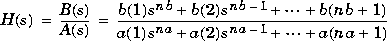
returns the real numerator and denominator coefficient vectors b and a of the transfer function

whose complex frequency response is given in vector h at the frequency points specified in vector w. Scalars nb and na specify the desired orders of the numerator and denominator polynomials.

Frequency is specified in radians between 0 and

, and the length of h must be the same as the length of w. invfreqs uses conj(h) at --w to ensure the proper frequency domain symmetry for a real filter.

[b,a] = invfreqs(h,w,nb,na,wt)

weights the fit-errors versus frequency. wt is a vector of weighting factors the same length as w.

invfreqs(h,w,nb,na,wt,iter)

and

invfreqs(h,w,nb,na,wt,iter,tol)

provide a superior algorithm that guarantees stability of the resulting linear system and searches for the best fit using a numerical, iterative scheme. The iter parameter tells invfreqs to end the iteration when the solution has converged, or after iter iterations, whichever comes first. invfreqs defines convergence as occurring when the norm of the (modified) gradient vector is less than tol. tol is an optional parameter that defaults to 0.01. To obtain a weight vector of all ones, use

invfreqs(h,w,nb,na,[],iter,tol)

invfreqs(h,w,nb,na,wt,iter,tol,'trace')

displays a textual progress report of the iteration.

invfreqs(h,w,'complex',nb,na,...)

creates a complex filter. In this case no symmetry is enforced, and the frequency is specified in radians between -

and

Remarks

When building higher order models using high frequencies, it is important to scale the frequencies, dividing by a factor such as half the highest frequency present in w, so as to obtain well conditioned values of a and b. This corresponds to a rescaling of time.

Examples

Convert a simple transfer function to frequency response data and then back to the original filter coefficients:

a = [1 2 3 2 1 4]; b = [1 2 3 2 3];
[h,w] = freqs(b,a,64);
[bb,aa] = invfreqs(h,w,4,5)
bb =
    1.0000    2.0000    3.0000    2.0000    3.0000
aa =
    1.0000    2.0000    3.0000    2.0000    1.0000    4.0000

Notice that bb and aa are equivalent to b and a, respectively. However, aa has poles in the left half-plane and thus the system is unstable. Use invfreqs's iterative algorithm to find a stable approximation to the system:

[bbb,aaa] = invfreqs(h,w,4,5,[],30)
bbb =
    0.6816    2.1015    2.6694    0.9113   -0.1218
aaa =
    1.0000    3.4676    7.4060    6.2102    2.5413    0.0001

Suppose you have two vectors, mag and phase, that contain magnitude and phase data gathered in a laboratory, and a third vector w of frequencies. You can convert the data into a continuous-time transfer function using invfreqs:

[b,a] = invfreqs(mag.*exp(j*phase),w,2,3);

Algorithm

By default, invfreqs uses an equation error method to identify the best model from the data. This finds b and a in

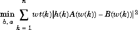
by creating a system of linear equations and solving them with MATLAB's \ operator. Here A(w(k)) and B(w(k)) are the Fourier transforms of the polynomials a and b, respectively, at the frequency w(k), and n is the number of frequency points (the length of h and w). This algorithm is based on Levi [1]. Several variants have been suggested in the literature, where the weighting function wt gives less attention to high frequencies.

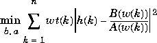
The superior ("output-error") algorithm uses the damped Gauss-Newton method for iterative search [2], with the output of the first algorithm as the initial estimate. This solves the direct problem of minimizing the weighted sum of the squared error between the actual and the desired frequency response points:

`freqs`	Frequency response of analog filters.
`freqz`	Frequency response of digital filters.
`invfreqz`	Discrete-time filter identification from frequency data.
`prony`	Prony's method for time domain IIR filter design.

References

[1] Levi, E.C. "Complex-Curve Fitting." IRE Trans. on Automatic Control. Vol. AC-4 (1959). Pgs. 37-44. [2] Dennis, J.E., Jr., and R.B. Schnabel. Numerical Methods for Unconstrained Optimization and Nonlinear Equations. Englewood Cliffs, NJ: Prentice Hall, 1983.