ugarchsim (Financial Toolbox)

Simulate a univariate GARCH(P,Q) process with Gaussian innovations.

Syntax

[U, H] = ugarchsim(Kappa, Alpha, Beta, NumSamples)

Arguments


`Kappa`	Scalar constant term of the GARCH process.
`Alpha`	`P`-by-`1` vector of coefficients, where `P` is the number of lags of the conditional variance included in the GARCH process. `Alpha` can be an empty matrix, in which case `P` is assumed `0`; when `P = 0`, a GARCH(0,Q) process is actually an ARCH(Q) process.
Beta	`Q`-by-`1` vector of coefficients, where `Q` is the number of lags of the squared innovations included in the GARCH process.
`NumSamples`	Positive, scalar integer indicating the number of samples of the innovations `U` and conditional variance `H` (see below) to simulate.

Description

[U, H] = ugarchsim(Kappa, Alpha, Beta, NumSamples)

Simulates a univariate GARCH(P,Q) process with Gaussian innovations.

U is a number of samples (NUMSAMPLES)-by-1 vector of innovations, representing a mean-zero, discrete-time stochastic process. The innovations time series U is designed to follow the GARCH(P,Q) process specified by the inputs Kappa, Alpha, and Beta.

H is a NUMSAMPLES-by-1 vector of the conditional variances corresponding to the innovations vector U. Note that U and H are the same length, and form a "matching" pair of vectors. To model the GARCH(P,Q) process, the conditional variance time series, H(t), must be constructed (see below). Thus, H(t) represents the time series inferred from the innovations time series vector U.

GARCH(P,Q) coefficients {Kappa, Alpha, Beta} are subject to constraints:

Kappa > 0
Alpha(i) >= 0 for i = 1,2,...P
Beta(i)  >= 0 for i = 1,2,...Q
sum(Alpha(i) + Beta(j)) < 1 for i = 1,2,...P and j = 1,2,...Q

The time-conditional variance, H(t), of a GARCH(P,Q) process is modeled as:

H(t) = Kappa + Alpha(1)*H(t-1) + Alpha(2)*H(t-2) +...+ Alpha(P)*H(t-P)+ Beta(1)*U^2(t-1)+ Beta(2)*U^2(t-2)+...+ Beta(Q)*U^2(t-Q)

Note that U is a vector of innovations, or regression residuals of an econometric model, representing a mean-zero, discrete-time stochastic process. That is, it is assumed that a regression model has already been run, and that U(t) = y(t) - F(X(t),B) is the time series of innovations derived from the model.

Although H is generated via the equation above, U and H are related as

U(t) = sqrt(H(t))*v(t)

where v(t) is an i.i.d. sequence ~ N(0,1).

The output vectors U and H are designed to be steady-state sequences; transients have arbitrarily small effect. The (arbitrary) metric used strips the first N samples of U and H such that the sum of the GARCH coefficients, excluding Kappa, raised to the N-th power, will not exceed 0.01:

       0.01 = (sum(Alpha) + sum(Beta))^N

Thus

       N = log(0.01)/log((sum(Alpha) + sum(Beta)))

Example

This example simulates a GARCH(P,Q) process with P = 2 and Q = 1.

% Set the random number generator seed for reproducability.
randn('seed', 10)
% Set the simulation parameters of GARCH(P,Q) = GARCH(2,1) process.
Kappa = 0.25;      %a positive scalar.
Alpha = [0.2 0.1]'; %a column vector of non-negative numbers (P = 2).
Beta = 0.4;        % Q = 1.
NumSamples = 500;  % number of samples to simulate.
% Now simulate the process.
[U , H] = ugarchsim(Kappa, Alpha, Beta, NumSamples);
% Now estimate the process parameters.
P = 2;    % Model order P (P = length of Alpha).
Q = 1;    % Model order Q (Q = length of Beta).
[k, a, b] = ugarch(U , P , Q);
disp(' ')
disp(' Estimated Coefficients:')
disp(' -----------------------')
disp([k; a; b])
disp(' ')
% Now forecast the conditional variance using the estimated   
% coefficients.
NumPeriods = 10;    % Forecast out to 10 periods.
[VarianceForecast, H1] = ugarchpred(U, k, a, b, NumPeriods);
disp(' Variance Forecasts:')
disp(' ------------------')
disp(VarianceForecast)
disp(' ')

When the above code is executed, the screen output looks like the display shown.

%%%%%%%%%%%%%%%%%%%%%%%%%%%%%%%%%%%%%%%%%%%%%%%%%%%%%%%%%%%

Diagnostic Information

Number of variables: 4

Functions 
Objective:        ugarchllf
Gradient:         finite-differencing
Hessian:          finite-differencing (or Quasi-Newton)

Constraints
Nonlinear constraints:             do not exist
Number of linear inequality constraints:    1
Number of linear equality constraints:      0
Number of lower bound constraints:          4
Number of upper bound constraints:          0
Algorithm selected
   medium-scale

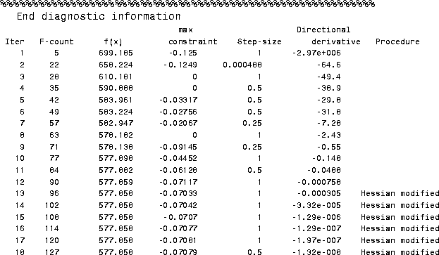
Optimization Converged Successfully
Magnitude of directional derivative in search direction 
  less than 2*options.TolFun and maximum constraint violation 
  is less than options.TolCon
No Active Constraints
Estimated Coefficients:
-----------------------
0.2520
0.0708
0.1623
0.4000
Variance Forecasts:
------------------
1.3243
0.9594
0.9186
0.8402
0.7966
0.7634
0.7407
0.7246
0.7133
0.7054