optexcit (Frequency Domain Identification Toolbox)

Generate the optimum input power spectrum for transfer function measurements.

X = optexcit(pdat,freqv)
[X,CR,fsv,vXwdev,Fiw] = ...
   optexcit(pdat,freqv,vdat,fixpind,X0,Ncyc,Fiw,pd)

Description

optexcit iterates towards the optimum power spectrum of the input signal in the sense that it minimizes the volume of the uncertainty ellipsoid of the estimated parameters of the linear system. The transfer function is given by pdat (the vector of all the parameters, see imppar; or a filename), the frequencies where the optimum spectrum is looked for are given in the vector freqv. The input and output variance vectors are given by vdat. If this is an 1-by-2 or 1-by-3 vector, its elements are taken as constant input and output variances, and may be the input-output covariance. If this is an N-by-2 or N-by-3 array, the variance vectors are formed from the first two columns, and the covariance vector from the third one; if this is a vector, the variance vectors and the covariance vector are obtained using impvar; if it is a string, the variance file is looked for.

fixpind defines the fixed parameters in the following way: if the parameters (numerator, denominator and the delay) are put together into a vector as: [num,denom,delay]', the elements of fixpind are the indices of the fixed parameters in this vector. (Here num and denom are row vectors defined in the usual way: in descending order of powers of s in the s-domain, or in ascending order of powers of z-1 in the z-domain.) When fixpind is given as just fixpind = 0, the zero-order coefficient of the denominator and the delay will be fixed. fixpind = 'n' means that there are no fixed parameters.

X0 contains the starting values of the amplitudes, and Ncyc gives the number of the iteration cycles. If Ncyc = 0, a "partial run" is performed, and the returned amplitude vector equals X0, but the Cramér-Rao bound CR is properly calculated. Fiw is a large array of partial information matrices, exported in a previous run for the same system for acceleration of the subsequent runs.

pd is the density of plots: plotting occurs if rem(cycle,pd) = 0, and in the last cycle. pd = inf will totally suppress plotting.

X is the generated amplitude vector. CR is the Cramér-Rao lower bound of the covariance matrix of the estimated parameters. For higher orders this matrix is usually very badly scaled in the s-domain, thus for the calculation of the determinant, scaling is advisable. fsv is the suggested scaling vector (CRscaled = CR.*(fsv*fsv')).

vXwdev is an 1-by-2 vector, containing the minimum and maximum deviations of the dispersion function from its limiting value, that is, the number of the free parameters.

Fiw is the above mentioned array. If Fiw is too large to be stored on the computer, it will be returned as empty array, and recalculated in every iteration cycle.

Important: The delay may also be estimated. Consequently, if it is fixed, it is to be given in fixpind.

A typical plot of optexcit is shown in the figure.

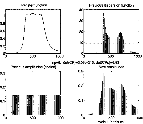The figure consists of four subplots. The first one shows the absolute value of the transfer function (linear scale), the one below it represents the previous amplitudes. The previous dispersion function shows the dispersion function calculated from the previous amplitudes. The result of the actual calculation cycle, the new amplitude set, is shown in the fourth subplot.

Below the dispersion function the number of free parameters is displayed (also represented by the dotted horizontal line in the plot). This is the theoretical final value of the dispersion function. The determinant of the covariance matrix, and the determinant of its scaled version are also shown.

Default Argument Values

vdat = [1,1].

Index vector of the fixed parameters: if fixpind is not given, in the s-domain

fixpind = [nn+nd,nn+nd+1],

that is, the coefficient of s0 in the denominator and the delay are fixed, while in the z-domain

fixpind = [nn+1,nn+nd+1]

the coefficient of z0 in the denominator and the delay are fixed. nn is the number of parameters in the numerator, nd is the same in the denominator. Note that fixpind = [] means that no fixed parameters are given (even the delay is variable); the default value can be given with fixpind = 0.

X0 = ones(F,1)/sqrt(F)

where F is the length of the frequency vector,

Ncyc = 1.

Examples

(see optexdem)

1.: Let us reproduce the results given in [1], Subsection 4.3.5, for a bandpass filter. After each power spectrum optimization step the crest factor is minimized, and the volume of CR is multiplied by an appropriate power of the crest factor.

: Some remarks concerning the program: optexcit is performed consecutively, but some rearrangement of the results was necessary because the routine produces the new amplitudes and the previous covariance matrix. Thus, crest factor minimization is performed on Xold. Moreover, msinclip is used in two steps: experience shows that it is advantageous to optimize first the input crest factor, and then use this result for input-output optimization.

num = [3.2010e-17,5.5155e-12,8.973e-10,0,0];
denom = [1.0131e-21,2.5351e-18,3.6031e-14,...
       5.5550e-11,3.5869e-7,2.5017e-4,1];
F = 50; fv = 20*[1:F]'; pd = exppar('s',num,denom);
fixpar = [4;5;12;13]; np = 9; Fiw =  '';
Xold = ones(F,1)/sqrt(F); Nold = 0;
for N = [1,2,3,4,10,11,100,101]
  [X,CR,fsv,vXwdev,Fiw] = ...
       optexcit(pd,fv,[1,1],fixpar,Xold,N-Nold,Fiw);
  tf = polyval(num,sqrt(-1)*freqv*2*pi)./...
       polyval(denom,sqrt(-1)*freqv*2*pi);
  [cx,crx,crxmax] = msinclip(fv,Xold, [],'lastgraph');
  [cx,crx,crxmax,cry,crymax] = ...
       msinclip(fv,cx,tf,'lastgraph');
  X = Xold; N = Nold;
  cyc = N-1, dCR = det(CR), crx, dCRs = dCR*crx^(2*np)
end %for N

2.: Let us check the theoretical results of the example given in [1] (Section 4.1, Example 2). A first order system is excited at just one frequency. The Cramér-Rao lower bound can be calculated in closed form (CRtheor), thus it can be compared to the covariance matrix given by the routine optexcit.

b0 = 1; b1 = 1; num = [1]; denom = [b1,b0]; f = 2;
parvect = exppar('s',num,denom);
cf = b0^2+(2*pi*f*b1)^2;
CRtheor = [cf*(1+cf)/(2*pi*f)^{2,0;0,cf*(1+cf)];
[X,CR] = optexcit(parvect,f,[1,1],[1,4],1,1);
format long e, CR, CRtheor

Diagnostics

The sizes of X0 and freqv must be equal, otherwise an error message is sent:

X0 has not the same size as freqv

If fixpind is given with value 0, a warning message is generated:

The denominator coefficient of s^0 and the delay will be fixed in optexcit

WARNING: the coefficient of z^0 and the delay will be fixed in optexcit

The variance vectors given by vdat must have the same length as fvect, otherwise an error message is sent:

The length of varx is ... instead of ...

Fiw is generated only if the computer can store it in full size. If this is not the case, Fiw will not be generated (this results in a longer run time. If Fiw is requested by defining it as an output argument, a warning message is sent:

WARNING! Fiw would be too large, it cannot be generated

and the output argument will be returned as an empty variable.

Algorithm

The algorithm is the one described in [1], [2] and [3]. First the partial information matrices are generated in each cycle for all the frequencies, then the dispersion function is determined, and the new power distribution is calculated.

References

[1] J. Schoukens and R. Pintelon, Identification of Linear Systems: a Practical Guideline for Accurate Modeling, London, Pergamon Press, 1991.
[2] F. Delbaen, "Optimizing the Determinant of a Positive Definite Matrix," Bulletin Société Mathématique de Belgique --Tijdschrift Belgisch Wiskundig Genootschap, Vol. 42, No. 3, pp. 333-346.
[3] K. R. Godfrey, ed.: Perturbation Signals for System Identification. Englewood Cliffs, Prentice-Hall, 1993.
[ Previous | Help Desk | Next ]