freqresp (Control System Toolbox)

Compute frequency response over grid of frequencies

Syntax

H = freqresp(sys,w)

Description

H = freqresp(sys,w)

computes the frequency response of the LTI model sys at the real frequency points specified by the vector w. The frequencies must be in radians/sec. For single LTI Models, freqresp(sys,w) returns a 3-D array H with the frequency as the last dimension (see "Arguments" below). For LTI arrays of size [Ny Nu S1 ... Sn], freqresp(sys,w) returns a [Ny-by-Nu-by-S1-by-...-by-Sn] length (w) array.

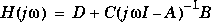
In continuous time, the response at a frequency

is the transfer function value at

. For state-space models, this value is given by

In discrete time, the real frequencies w(1),..., w(N) are mapped to points on the unit circle using the transformation

where

is the sample time. The transfer function is then evaluated at the resulting

values. The default

is used for models with unspecified sample time.

Remark

If sys is an FRD model, freqresp(sys,w), w can only include frequencies in sys.frequency.

Arguments

The output argument H is a 3-D array with dimensions

For SISO systems, H(1,1,k) gives the scalar response at the frequency w(k). For MIMO systems, the frequency response at w(k) is H(:,:,k), a matrix with as many rows as outputs and as many columns as inputs.

Example

Compute the frequency response of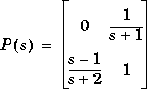

at the frequencies

. Type

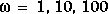
w = [1 10 100]
H = freqresp(P,w)
H(:,:,1) =
 
        0            0.5000- 0.5000i
  -0.2000+ 0.6000i   1.0000         
 
 
H(:,:,2) =
 
        0            0.0099- 0.0990i
   0.9423+ 0.2885i   1.0000         
 
 
H(:,:,3) =
 
        0            0.0001- 0.0100i
   0.9994+ 0.0300i   1.0000

The three displayed matrices are the values of

for

The third index in the 3-D array H is relative to the frequency vector w, so you can extract the frequency response at

rad/sec by

H(:,:,w==10)

ans =
        0            0.0099- 0.0990i
   0.9423+ 0.2885i   1.0000

Algorithm

For transfer functions or zero-pole-gain models, freqresp evaluates the numerator(s) and denominator(s) at the specified frequency points. For continuous-time state-space models

, the frequency response is

When numerically safe,

is diagonalized for fast evaluation of this expression at the frequencies

. Otherwise,

is reduced to upper Hessenberg form and the linear equation

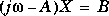is solved at each frequency point, taking advantage of the Hessenberg structure. The reduction to Hessenberg form provides a good compromise between efficiency and reliability. See [1] for more details on this technique.

Diagnostics

If the system has a pole on the

axis (or unit circle in the discrete-time case) and w happens to contain this frequency point, the gain is infinite,

is singular, and freqresp produces the following warning message.

Singularity in freq. response due to jw-axis or unit circle pole.

References

[1] Laub, A.J., "Efficient Multivariable Frequency Response Computations," IEEE Transactions on Automatic Control, AC-26 (1981), pp. 407-408.