ATLAS
FLORAE EUROPAEAE
Old Grid System
The grid of Atlas Florae Europaeae volumes 1 - 12, with its
4419 grid cells, was modified from the Military Grid Reference
System (MGRS). The MGRS itself is an alphanumeric version of a
numerical UTM (Universal Transverse Mercator) or UPS (Universal
Polar Stereographic) grid coordinate.
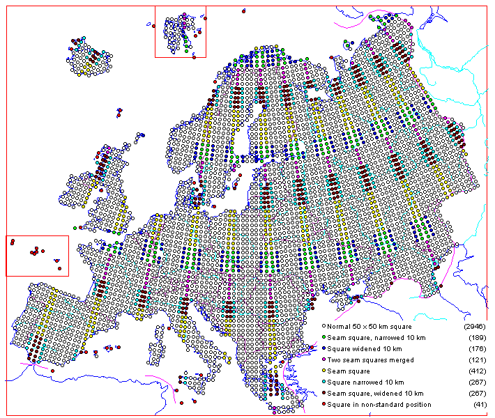
AFE 1 - 12 used the 50 x 50 km quadrants of the MGRS 100 x 100
km squares as mapping units. The MGRS pattern was modified in AFE
as follows:
- Numbers 1 to 4 to indicate the 50 km x 50 km quarters of
the MGRS 100 km x 100 km squares. This coding, such as
MG1, MG2, MG3 and MG4 (for the NW, SW, NE and SE quarters
of the larger MGRS squares), is not supported by the
MGRS.
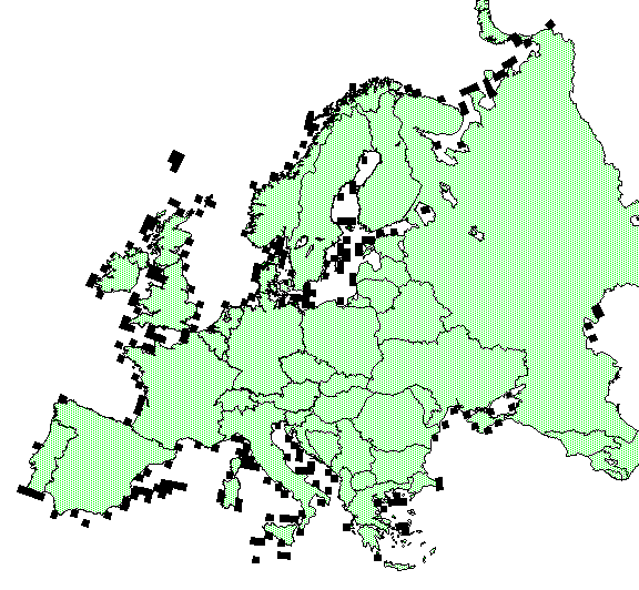
Black squares in the picture above indicate grid cells which were
not used. The records from them were moved to adjacent squares,
or to grid cells in non-standard position. Iceland, Svalbard and
Azores not illustrated (there are plenty of similar cases in
those areas, too).
- In coastal areas the squares with less than 10 % (250 km2)
of land, records were transferred into the nearest
mainland square. However, islands far from the coast and
long peninsulas had their own squares. Some of the
deviations are listed below:
An asterisk
(*) indicates symbols of squares the circles of which
deviate from the actual position of the UTM squares.
|
British Isles
|
The entire S. Part of the Isle of Lewis is in
PE2.
All of North Uist (etc.) is in *ND3.
All of S. South Uist (Barra, etc.) is in *ND4.
Dunvegan Head is in PD3.
All of the Isle of Man is in *UF4.
All of the Scilly Isles are in PR4.
UA2 is included in *UA1.
UA4 is included in UA3.
Guernsey and Sark are in WV1.
Alderney and Jersey are in WV3.
|
Denmark
|
All of Laesö is in *PJ1.
All of Bornholm is in *VB4.
Faeröerne are in *FaeN and *FaeS, the limit between them
follows Skopen Fjord.
|
Germany
|
Helgoland is in ME1.
VA2 contains only E. Rügen.
|
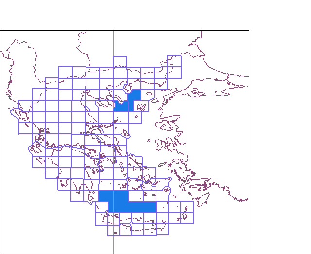
Greece
|
The scheme from AFE vol. 3 (1976):
|
Iceland
|
All of Snaefellsnes is in *AN4.
|
Italy
|
NP4 is included in PP2.
*PN2 contains: all of Elba, Capraia, Pianosa,
Montecristo, and islands W. Of it. (Mainland on PN2 is
included in PN4).
UF2 also contains islands of UF4.
All of Isole Eolie o Lipari are in *VC3.
All of Pantelleria is in *QF3.
All of Isole Pelagie are in *TV1.
(All of Malta is in *VV1).
|
Netherlands
|
All of Vlieland is in FU1.
All of Terschelling is in FV4.
|
Norway
|
Kjelmesöy and the peninsula E. Of it are in
VC2.
*Björnöya and *Jan Mayen form a square of their own.
Kvitöya is in *NK4.
Kongsöya is in *NH1.
Svensköya is in *MH4.
Hopen is in *MF4.
|
Portugal
|
Each island of the *Azores forms a square of its
own.
|
Russia
|
All of Poluostrov Rybachiy is in VC4.
NW. Kanin is in *MB4.
Ostrov Matveyev is in EB3, the rest of EC4 is included in
EC3.
All of Sur Sari is in NG1.
Ostrov Malyy Tyutyarsari is in NG2.
Kolka is in EJ3.
Ostrov Dzharylgach is in VS4, Rybnoye in VR4.
|
Spain
|
BD2 is included in *BC1.
All of Isla of Ibiza is in *CD4.
The entire W. part of Isla de Mallorca is in *DD3, the E.
part in *ED1.
All of Isla de Menorca is in *EE4.
I. Alboran is in *VE3.
|
Sweden
|
All of Gotska Sandön is in *CK3.
All of Central Gotland is in *CJ1.
W. edge of XD1 is in WD3, N. Öland is in XD2.
|
Turkey (European part)
|
All of Imroz Ada is in ME2.
PF4 is included in *PF3.
|
- The centre of grids covering isolated islands was put to
the actual position of the island, irrespective of the
standard grid. This resulted also in
"polygon-like" grid cells, to include whole
islands in a particular square.
- Certain individual mountain tops forming distinct
biogeographic entities were not divided between two or
more squares, despite of the grid.
- The square codes for all of Iceland deviated from the
MGRS pattern.
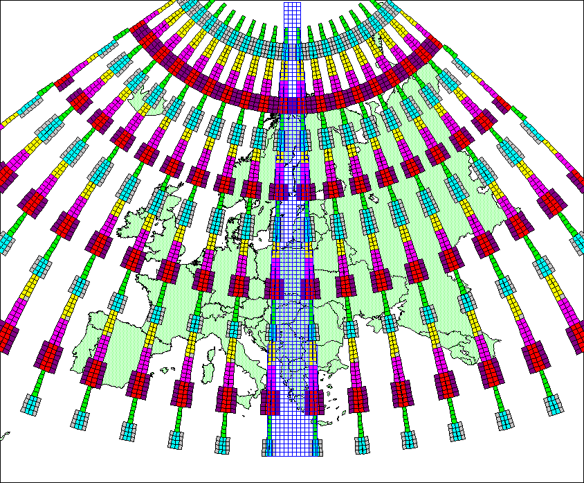
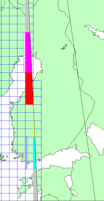
AFE grid pattern (not the actual grid; grid deviations
omitted from this picture). Pale green = central seam square
(two MGRS squares of different UTM zones merged, base width of
the squares between 20-30 km); pale blue = seam square, widened
for 10 km (base width 30-40 km); yellow = seam square with base
width over 40 km; purple = narrow seam square (base width < 10
km merged with adjacent square in the same zone); red = seam
square, narrowed 10 km; grey = rectanangular square, width 60 km;
dark violet = rectangular square, base width 40 km; blue
gridlines = MGRS grid in the UTM zone 34
- To be able to limit the longitudinal width variation of
the grid cells to 40 to 60 km, in the overlapping area
between different UTM zones, the longitudinal limits of
the grid cells were shifted outwards or inwards. When the
standard MGRS squares extended into adjacent UTM zone,
they were treated differently depending on the distance
between the UTM zone boundary and the SW corner (if the
square belongs to the zone west of the zone boundary) or
SE corner (if in the eastern zone) of such seam squares.
That distance, let's call it "x" below, is
something between 0 - slightly above 50 km (can be above
50 in some cases, for instance where a UTM zone boundary
goes through the NE corner of a square at the zone
border). The x values of 10, 20, 30, 40 kilometers
influenced the treatment of the squares in AFE 1 - 12
this way:
|
Eastern border of the UTM zone 34 in
Estonia and Finland.
|
- GREY = Parts of squares on the
different sides of the zone boundary are merged
if 40 <= x + x <= 60 km. This means for the
squares to be merged, x must be between 20 and 30
km. Standard 10-km UTM lines are followed here,
and the merging has no effect on the width of the
adjacent standard squares.
- CYAN (DENSE BLUE DIAGONAL GRID
SHOWS HOW THE WIDTH OF THE ADJACENT SQUARE IS
CHANGED). If x is less than 20 km, the squares on
different sides of the zone boundary are not
merged, but the small parts of seam squares are
joined the adjacent standard square. In cases
where this would result in squares wider than 60
km, the width of the adjacent standard square is
adjusted by narrowing its western or eastern edge
(the edge farther from the zone border) to the
next full 10-km UTM easting. In these cases x +
50 <= 60 which means if x is between 10 and
20, this longitudinal shift affecting the width
of adjacent standard squares is done. Thus the
width of the next standard square also grows to
60 km.
- YELLOW = If x is below 10 km, then
slices are joined to the adjacent square without
additionally reducing its width by 10 kilometers
(and thus the next square remains as 50 km x 50
km square). Thus the width of the adjacent
standard squares becomes something between 50 and
60 km.
- PURPLE (PURPLE HORIZONTAL GRID
SHOWS HOW THE WIDTH OF THE ADJACENT SQUARE IS
CHANGED). If x is more than 30 km, but less than
40 km, the partial square are not joined to the
adjacent standard square, they would become too
wide. Instead the edge outwards of the zone is
extended to the next full 10-km UTM easting. Thus
the grid cells become at least 40 km wide.
Simultaneously the adjacent standard squares
become 10 km narrower.
- RED = If x is more than 40 km, the
square is treated as an independent grid cell.
|
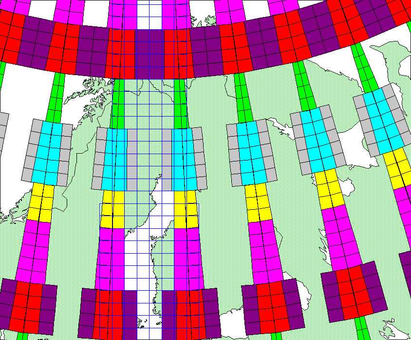
AFE old grid pattern in N Europe (deviations
from the general pattern not shown!).
References: