Now that you have some working knowledge of what a GIS can do, consider next some of the actual mechanics of conducting a GIS analysis. Today, this is done almost exclusively on computers. Typical hardware in current use is depicted in this diagram:

From B. Davis, GIS: A Visual Approach, ©1996. Reproduced by permission of Onword Press, Santa Fe, NM.

Many software packages for GIS analysis have been developed. The most widely used are ARC/INFO (Unix and Windows NT platforms) and ArcView (a smaller PC desktop version) marketed by the Environmental Systems Research Institute (ESRI) of Redlands, California, a company founded in 1969 by Jack and Laura Dangermond. A tutorial on the use of ARC/INFO (http://boris.qub.ac.uk/shane/arc/ARChome.html) has been put together by Shane Murnion of Queens University in Belfast. Another well-known program, developed by the U.S. Army Corp of Engineers, and in the public domain, is GRASS (http://www.cecer.army.mil/grass/GRASS.main.html), an acronym for Geographic Resources Analysis Support System), for which a tutorial centered on a case study is found at a site (http:// severn.geog.le.ac.uk/assist/grass/seeds/gs_intro.html) maintained by the University of Leicester in England.

The following flow diagram outlines a general system design for procedures and steps in a typical GIS data handling routine:

The objective in this operation is to assemble a data base that contains all the ingredients needed to manipulate through models and other decision-making procedures into a series of outputs applicable to the problem-solving effort.

Some input data may already exist in digital form but most must be converted from maps and tables or other sources into this form. Some maps or satellite/aerial imagery can be scanned and the resulting products handled as digital inputs using individual pixels that are data cell equivalents (note that the pixels are directly recorded as colors; these values must be recoded if they are to be associated with specific attributes). Although recent technology has permitted this conversion to be automated, it is still true in many instances that maps in particular must be digitized manually, using a digitizing board or tablet, such as shown here:

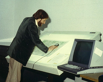
Behind this table, on which a map is mounted, are closely spaced electrical wires arranged in a criss-cross pattern which forms a grid that can be referenced as x-y coordinates. A mobile puck (in Bill Campbell's [author of the afore-referenced chapter on GIS in the Landsat Tutorial Workbook] right hand) with centered crosshairs is placed over any point on the map, a button clicked, and its position entered into a computer base, along with some numerical code that records its attribute(s).

Any map consists of points, lines, and polygons that locate individual spots or enclose patterns (information fields) that describe particular attributes or theme categories. Consider this situation that refers to several fields (e.g., different types of vegetation cover) separated by linear boundaries:

The information contained in each field can be captured by either of two methods of geocoding: Vector or Raster. In the central panel, the approach is that of creating polygons comprised of some number of straight lines that approximate the curvature of the field (if that field has irregular boundaries, many lines may be needed). Each line consists of two end points (a vector) whose positions are marked by coordinates during digitizing. That process is indicated in this diagram:

From B.Davis, GIS: A Visual Approach, ©1996. Reproduced by permission of Onword Press, Santa Fe, NM.

Each point has a unique coordinate value. A line is defined by two ends or node points, each with its coordinates. A polygon is specified by a series of connecting nodes (any two adjacent lines share a node) which must achieve proper closure (in the writer's experience with digitizing, the main pitfall is that when an array of polygons is checked out, some failure to close seems inevitable and the process may need repeating or at least repair). Each polygon is then identified by a proper code label (numerical or alphabetic; the code characters can be associated with the attributes they represent through a look-up table). In this way, all map fields large enough to be conveniently circumscribed and their category values can be entered into a digital database.

In the raster approach, a grid array of cells having some specific size is overlain manually or by scanning on to the map. As shown in the right panel (grid format) two figures above, an irregular polygon will then include some number of cells completely contained therein. These are recorded as to location within the grid and the relevant code number for each data element assigned to them. But some cells will straddle field boundaries; a preset rule assigns the cell to one or the other of adjacent fields, usually according to some rule related to the relevant proportion of either field. The array of cells that cluster about a field will be only an approximation of the field shape but for most purposes the inaccuracy introduced is tolerable for calculation purposes. Generally, grid cell dimensions are greater than those of enclosed pixels in pictorial displays of the maps but again the cluster of pixels within the same polygon approximates the shape of the field. This raster format is well adapted to digital manipulation because of the relation of cells to this pixel subdivision. The size of a cell is partly dependent on the internal variability of the feature or property being represented; smaller cells increase accuracy but also require more data storage. Note that multiple data layers referenced to the same grid cell base will share this spatial dimensionality but will have different coded values for the various attributes associated with any given cell.

Data management is sensitive to storage retrieval methodology and to file structures. A good management software package should be able to:

1. Scale and rotate coordinate values for "best fit" projection overlays and changes.
   
   
2. Convert (interchange) between polygon and grid formats.
   
   
3. Permit rapid updating, allowing data changes with relative ease.
   
   
4. Allow for multiple users and multiple interactions between compatible data bases.
   
   
5. Retrieve, transform, and combine data elements efficiently.
   
   
6. Search, identify, and route a variety of different data items and score these values with assigned weighted values to facilitate proximity and routing analysis.
   
   
7. Perform statistical analysis, such as multivariate regression, correlations, etc.
   
   
8. Overlay one file variable onto another, i.e., map superpositioning.
   
   
9. Measure area, distance, and association between points and fields.
   
   
10. Model and simulate, and formulate predictive scenarios, in a fashion that allows for direct interactions between the user group and the computer program.
    
    

The development of a GIS can be a costly, complex, and somewhat frustrating experience for the novitiate. It should be stressed that data base design and encoding are major tasks that demand time, skilled personnel, and adequate funds. However, once developed, the information possibilities are exciting, and the marginal costs of handling the various kinds of data are more than compensated for by the intrinsic worth of the output. In plain language, GIS has obvious payoffs in the systematic, versatile, and comprehensive way in which spatial (geographic) data are presented, interpreted and recast in intelligible output.

---

[an error occurred while processing this directive] [an error occurred while processing this directive]