Some elements of the above ideas were brought home to the author during his first experience in the late summer of 1974 while going into the field to check on an unsupervised classification made by the LARSYS (Purdue University) processing system and to designate new training sites for a subsequent supervised one. The classified area was centered on glacial Willow Lake on the southwestern flank of the Wind River Mountains of west-central Wyoming. Prior to arriving onsite, a series of computer-generated printouts (long since misplaced), in which each spectral class (separable statistically but not identified) was represented by its own alphanumeric symbol, had been prepared. Different clusters of the same symbols suggested that discrete land use/cover classes were present. In the processing, the total number of classes was allowed to vary. Printouts with 7 to 10 such classes looked most realistic. But there was no a priori way to decide which was most accurate. In touring the area, preconceived notions about classes had to be revised or modified. The importance of grasses and of sagebrush had not be considered, and the presence of clumps of trees below the 79 m (259 ft) resolution of the Landsat MSS was not anticipated. After a tour through the site, the author gazed over the scene from a slope top and tried to fit the patterns in the different maps into the distribution of features on the ground. The result was convincing: the 8 class map was mildly superior to the others. Without this bit of "ground truthing", it would have been difficult to feel any confidence in interpreting the map and deriving any measure of its accuracy. Instead, what happened was a "proofing" of reliability for a mapped area of more than 25 square kilometers (~10 square miles) through a field check of only a fraction of that area.

Accuracy may be defined, in a working sense, as the degree (often as a percentage) of correspondence between observation and reality. Accuracy is usually judged against existing maps, large scale aerial photos, or field checks. Two fundamental questions about accuracy can be posed: Is each category in a classification really present at the points specified on a map? Are the boundaries separating categories valid as located? Various types of errors diminish accuracy of feature identification and category distribution. Most are made either in measurement or in sampling. Three error types dominate:

1. Data Acquisition Errors: These include sensor performance, stability of the platform, and conditions of viewing. They can be reduced or compensated by making systematic corrections (e.g., by calibrating detector response with on-board light sources generating known radiances). Corrections, often modified by ancillary data such as known atmospheric conditions during overpass, can be made during initial processing of raw data.

2. Data Processing Errors: An example is possible misregistration of equivalent pixels in the different bands of the Landsat Thematic Mapper. The goal in geometric correction is to hold the mismatch to a displacement of no more than 1 pixel. Under ideal conditions, and with as many as 25 ground control points (GCP) spread around a scene, this goal can be realized. Misregistrations of several pixels significantly compromise accuracy.

3. Scene-dependent Errors: As alluded to in the previous page, one such error relates to how the class is defined and established which, in turn, is sensitive to the resolution of both the observing system and the reference map or photo. Three variants of these are exemplified by a common geologic situation (also treated to some extent in Section 2) in which the sensor data are processed primarily to recognize rock types at the surface. In this there are pitfalls. First, geologists in the field seek to map bedrock but over large parts of a surface, soil and vegetation cover mask the bedrock at many places. The geologist makes logical deductions in the field as to the rock type most likely buried under the surface and shows this on a map (in which these masking materials are treated as invisible [ignored]). This, unfortunately, does not correspond to what the sensor "sees". Second, most geologic maps are stratigraphic rather than lithologic, i.e., consist of units identified by age rather than rock type. Thus, the same or similar rock types will be shown by different symbols or colors on the map, so that checking for ground truth requires conversion to lithologies (often difficult because a unit may be diverse lithologically but was chosen for some other mode of uniformity). Third, a rock type may need to be considered in context with its surroundings in order to be properly named. Granite, and the sedimentary rock called arkose derived from it, both have similar spectral properties. The latter, however, typically is arranged in strata, being distributed as a depositional formation, whose spatial patterns (especially when exposed as folded or inclined layers) are usually quite distinct from those of massive granites and are often revealed by topographic expression.

As a general rule, the level of accuracy obtainable in a remote sensing classification depends on such diverse factors as the suitability of training sites, the size, shape, distribution, and frequency of occurrence of individual areas assigned to each class, the sensor performance and resolution, and the methods involved in classifying (visual photointerpretation versus computer-aided statistical classifier), and others. A quantitative measure of the mutual role of improved spatial resolution and size of target on decreasing errors appears in this plot:

The dramatic improvement in error reduction around 30 m (100 ft) is related in part to the nature of the target classes - coarse resolution is ineffective in distinguishing crop types but high resolution (< 20 m) adds little in recognizing these other than perhaps identifying species. As the size of crop fields increases, the error decreases further. The anomalous trend for forests (maximum error at high resolution) may (?) be the consequence of the dictum: "Can't see the forest for the trees." - here meaning that high resolution begins to display individual species and breaks in the canopy that can confuse the integrity of the class "forest". Two opposing trends influence the behavior of these error curves: 1) statistical variance of the spectral response values decreases whereas 2) the proportion of mixed pixels increases with lower resolution.

A study of classification accuracy as a function of number of spectral bands shows this:

The increase from 1 to 2 bands produces the largest improvement in accuracy. After about 4 bands the accuracy increase flattens or increases very slowly. Thus, extra bands may be redundant, as band-to-band changes are cross-correlated (this correlation may be minimized and even put to advantage through Principal Components Analysis). However, additional bands, such as TM 5 and 7, can be helpful in rock type (geology) identification because compositional absorption features diagnostic of different types reside in these spectral intervals. Note that highest accuracy associates with crop types because fields, consisting of regularly-space rows of plants against a background of soil, tend to be more uniform .

In practice, accuracy of classification may be tested in four ways: 1) field checks at selected points (usually non-rigorous and subjective) chosen either at random or along a grid; 2) estimate (non-rigorous) of agreement on theme or class identify between class map and reference maps, determinedusually by overlaying one on the other(s); 3) statistical analysis (rigorous) of numerical data developed in sampling, measuring, and processing data, using such tests as root mean square, standard error, analysis of variance, correlation coefficients, linear or multiple regression analysis, and Chi-square testing (see any standard text on statistics for explanation of these tests); and 4) confusion matrix calculations (rigorous). This last approach is best explained by the writer's study made of a subscene from a July, 1977 Landsat image that includes Elkton, Maryland (top center).

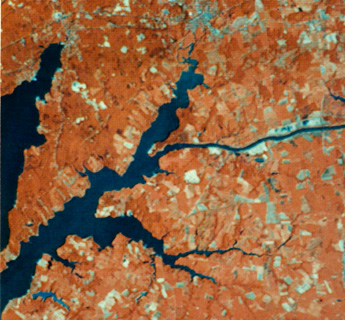
A 1:24,000 aerial photo that falls within this subscene was acquired from the EPA. Starting with a field visit in August, 1977 during the same growing season as the July overpass, the crops in many individual farms located in the photo were identified, of which about 12 were selected as training sites. Most were either corn or soybeans; others were mainly barley and wheat. A Maximum Likelihood supervised classification was then run, as shown below,

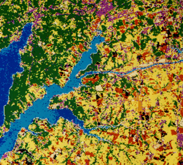
and printed out as a transparency; This was overlaid on to a rescaled aerial photo until field patterns approximately matched. With the class identities in the photo as the standard, the number of pixels correctly assigned to each class and those misassigned to other classes were arranged in the confusion matrix used to produce the summary information shown in Table 13-2, listing errors of commission, omission, and overall accuracies.

Errors of commission result when pixels associated with a class are incorrectly identified as other classes, or from improperly separating a single class into two or more classes. Errors of omission occur whenever pixels that should have been identified as belonging to a particular class were simply not recognized as present. Mapping accuracy for each class is stated as the number of correctly identified pixels within the total in the displayed area divided by that number plus error pixels of commission and omission. To illustrate, in the table, of the 43 pixels classed as corn by photointerpretation and ground checks, 25 of these were assigned to corn in the Landsat classification, leaving 18/43 = 42% as the error of omission; likewise, of the 43, 7 were improperly identified as other than corn, producing a commission error of 16%. Once these errors are determined by reference to "ground truth", they can be reduced by selecting new training sites and reclassifying, by renaming classes or creating new ones, by combining them, or by using different classifiers. With each set of changes, the classification procedure is iterated until a final level of acceptable accuracy is reached.

---

[an error occurred while processing this directive] [an error occurred while processing this directive]