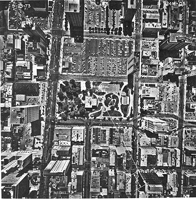
Both heights of surface features (e.g., tall trees and buildings) and relief can be measured by various photogrammetric techniques. Consider for example the determination of the height h of a tall building that lies near the edge of a single aerial photograph. If that photo was taken as truly vertical, i.e., looking straight down, then its center lies at the nadir (the vertical line from camera perpendicular to a surface point directly beneath [assumed to be flat ]). In that instance, the nadir coincides with the principal point (p.p.) in the photo which is the intersection of the lens' optical axis (as though extended) and the ground, so that the p.p. is also the true center of the photo; that point becomes off-center if the photo (and optical axis) is non-vertical. If the building were to lie close to the p.p., its top and bottom would appear to coincide in the photo. If it is well away from that point at some radial distance r towards the edge, its viewed state at a slant would have the top displaced further away from the p.p. than the bottom by some amount measurable in the photo as d. For an aircraft height H (calculable from the scale if a ground distance is known), the value of h is just: h = (d/r) x (H). This approach can be illustrated with a large scale, low camera altitude aerial photo of the downtown area of Long Beach, California (from Sabins, 1987; courtesy J. Van Eden), in which the lateral tilt of tall buildings is obvious in the outer parts; d and r have been drawn between the p.p. and one of the buildings near the edge:

Height differences [relief] between points of different elevation along surfaces can be calculated from stereo pairs using this formula: h = (H) dP/(P + dP). Cross-check the figure above figure and the drawing below as an aid to visualizing the process (the two photos in the drawing are shown as "cockeyed", typical of the effects of inflight yawing [rotation around a vertical axis]).

P is the absolute stereo parallax. For any standing object or separated points on a slope whose height or relief is to be determined, the distance (in the direction parallel to the flight line) on one photo between the base (here: point b) of that feature and the principal point (PP1) or nadir is measured. The same is then done for that conjugate feature as it appears in some different position in the other photo (note that the first photo p.p.[pp1] now lies at some distance off-center [at pp1'] from the second photo p.p. [pp2]) and averaging the two distances (d₁ + d₂ divided by 2). The dP term is the differential parallax: it is determined by measuring the distance between the base and the top of the feature or between two proximate terrain points at different elevations on a slope as located in each of the two photos when the pair is in optimum alignment for stereo viewing; dP then is the numerical difference between the two distance values (x₂ - x₁) which will be different in each of the photo pair.The value of dP is established optically through use of special devices such as a stereometer, a parallax wedge, or, most commonly, a parallax bar. Each uses a variant of the "floating point" method in which reference marks - dot or cross - are visible when the aligned photos are viewed under a mirror stereoscope. The parallax bar is placed on the photo plane so that a fixed mark over one photo is made to coincide with a movable mark (fused visibly in the stereo view) by turning a screw drive that translates that mark into coincidence; the value of dP is then read from a graduated scale. When this is done for a number of points, heights and relief values for parts of the map can be calculated; these become absolute values (elevations) if points are referenced to benchmarks.

Use of the above devices to specify a large enough number of elevation points in stereo photos to permit contouring is difficult and tedious. Sophisticated optical-mechanical stereoplotters are applied instead. These use two or three movable projectors that pass light through stereo pairs made into glass-mounted film diapositives placed onto a tracing table (platen) which can be raised and lowered. A 3-D image or stereomodel is produced which can be viewed by an outside observer by some filter method (for black and white photos, this is done by the anaglyph method in which one photo is projected through a red filter and the other a cyan filter and then viewed through eyeglasses with corresponding color filters). A small point of light or dot is projected onto the stereomodel. When the dot appears to coincide with some part of the model surface (as seen through the viewer), that dot locates a particular elevation determined by the platen height and calibrated by control points. An experienced operator can then move the light along the model surface such that it always remains coincident. This motion traces a contour line. The platen table is then raised (or lower) a fixed amount determined by the contour interval chosen and the next elevation is contoured, and so on until the entire surface is thus traced. Today, analytical stereoplotters are capable of semi-automating the contouring through computer processing of mathematically transformed data.

A general review of the concepts and mechanics of producing DEMs can be accessed at a site maintained by the Eros Data Center (EDC). http://edcwww.cr.usgs.gov/glis/hyper/guide/usgs_dem

---

[an error occurred while processing this directive] [an error occurred while processing this directive]