You can deduce from the table on the previous page, that, dependent on the actual standard deviations (not shown), most of the signatures have combinations of DN values that would appear to allow their distinctions from one another. Two classes - Urban 1 and Cleared [Ground] - are quite similar in the first four bands but apparently are different enough in bands 5 and 7 to suppose that they are separable. The range of variations in the thermal band 6 is much smaller than in other bands, suggesting its limitation as an efficient separator. However, as will be seen below, its addition to the Maximum Likelihood Classification increases the spatial homogeneity of some classifications
Minimum Distance Classification
We initiate our survey of supervised classification by producing
one using the minimum distance routine. The Idrisi program acts on DNs in multidimensional band
space to organize the pixels into the classes chosen. Each "unknown"
pixel is then placed in the class closest to the mean vector in this band space. For Morro Bay, the resulting
classification image consists of 16 gray levels, each representing
a class, that can then be assigned on the computer any color one
wishes; combinations are usually selected to have either color
themes (similar colors for related classes) and/or to set spatially
adjacent classes apart to the eye by using disparate colors. Examine
this minimum distance classification,
in which all 7 TM bands including the thermal participate. Study it in relation to your acquired knowledge of this scene from the preceding pages in this section and compare it with the classification we will now show.
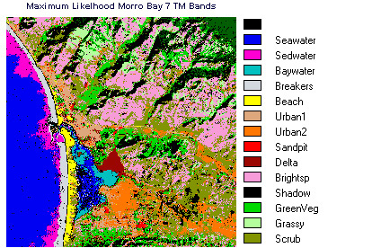
Maximum Likelihood Classification
This next supervised classification is made using the maximum
likelihood classifier. Again, multiband classes are statistically
derived and each unknown pixel is probabilistically analyzed to
evaluate which class it has the highest likelihood of belonging
to. In the image next displayed thermal band 6 is omitted and
16 classes are defined (this is the maximum allowable in the Idrisi
program). These are identical to the previous ones recorded in
the minimum distance image. In both instances, the sediment has
been subdivided into three levels (I and II in the ocean and a
third in the Bay) and two urban classes (I = Morro Bay; II = Los
Osos) are attempted to account for visual differences between
them (mainly street patterns). Look at this image classification
and judge for yourself how believable is the result. Compare it with the minimum distance image as well; to assist you in equating similar classes, the same color assignments are shared. Then, look at a supervised classification
using Band 6 and again specifying 16 classes; note how each urban area becomes more homogeneous. Similar increase in spatial homogeneity of vegetation and generalized slopes is noted with band 6 added, but overall the differences between With and Without 6 are rather slight.
Your first impression is that each 16 class maximum likelihood version is a fairly dazzling image, with many classes "right on". Both breakers and sand bar (beach) seem uniformly classified. The sediment load distribution is credible. There are enough color tone differences between Morro Bay and Los Osos to justify the decision to set them up as two classes (Los Osos differs in its street patterns and in the presence of the orange-brown "soil" seen in the 1,2,3 composite) but color elements of one urban class are mixed with the other, in differing proportions, as one would expect. The bright orange given to the coastal marsh area occupies a slightly larger area than its equivalent does in the minimum distance classification and is also distributed in small patches around the Los Osos coastline, and again along the river (p) - probably a true condition in that such vegetation should be more widespread. No doubt the most uncertain group of classes is spread over the hills. The categories Sun Lit Slope and Shadow Slope are somewhat synthetic in that they refer mostly to an illumination condition whereas the classes grass and trees may be a mix of lighting effects and actually a lighter or darker surface. The class Cleared Land is again both a depiction of land surfaces that may support not only thin natural vegetation or even be partially barren but also may in some places again be a shadowing effect. The Grasslands is properly placed in this image but appears to spread over wider areas than indicated in several other images - this is doubtless a valid case. The Green Vegetation category proxies well for the actual distribution of reflective organic material (in band 4) but in this choice of class assignments the several types of growing ground cover are not singled out. Thus, elements of the golf course and the mountain crest forest are shown as "like" and are not distinguished from field crops, etc. They could have been told apart to some degree of "correctness" if each had been given its own class and training sites selected.
Nearly two years after the above supervised classifications were
executed, an occasion arose to re-do the same scene using new
Idrisi software that operates from Windows rather than DOS 3.1.
(that was on Windows Version 1; Version 2 is now available). In
performing this supervised classification, the same Maximum Likelihood
classifier was used with all 7 TM Bands and again 15 classes were
set up. But, as an experiment, it was decided to drop several
class categories and select new ones instead. Also, somewhat different
training site polygons were established for each class. In effect,
this achieved an independent classification without "peeking"
at the results shown above for guidance. And, instead of using
the natural color scene from which to pick training sites, the
false color image was employed. This is the result:
Note that for nearly all classes different colors were assigned
which makes it rather difficult to compare the results with the
earlier classifications. In the above image, one of the classes
is omitted from the Legend (a quirk of the image display in this
Windows version); it is the class Trees, which is rendered in
Dark Green. Nevertheless, scrolling back and forth between this
and the 7 band Supervised Classification just above reveals both
differences and similarities.
In the Windows version, the two sediment classes have been combined.
Also, the class called Fields in the 3.1 version is here renamed
GreenVeg and includes not only fields in crop but also some natural
vegetation (probably local woodlands); both show as bright red
in the false color rendition. The Trees distribution is similar
in both classifications but is a bit more widespread in the Windows
version (but harder to see because dark green and black shadows
do not single out in good contrast). The classes Scrubland and
Cleared in the 3.1 version are partially represented by Scrub
in the Windows version. In 3.1, Urban II (trained on the street
pattern in Los Osos) is olive and is orange in the Windows version;
in both cases, the distribution of the Urban II class pattern
is much more extensive than is the real situation. Towns or clusters
of buildings do not exist in the long orange strip near the highway
nor in the lower right part of the image. Apparently, some natural
surfaces, as interpreted just from the true and false color composite
images, give rise to signatures that resemble this urban class.
In the Windows version, several very bright areas, mainly around
Los Osos, have been named Sandpit. This is a guess: they may be
excavated ground or inland remnants of beach sand (although they
classify as distinct from the Sand Class); only an on-site visit
could ascertain a correct identity. The point in running and comparing
these two classifications is probably obvious: the precise end
result - mainly in extrapolating classes from their training sites
to the identities and distribution of the selected classes, i.e.,
the overall appearance and accuracy of the classification - is
sensitive to the variables involved and the choices made. Interpretations
will differ depending on the colors and other factors present
in the training image by which the classes are chosen as separable
and efficient training sites blocked out. The number of classes
sought, the validity (purity) of the enclosed space representing
these classes in the training sites (and the number of pixels
in the polygons assigned to each class), the nature of a class
(the urban division is somewhat artificial; scrub may in fact
be composed of rather dissimilar classes or features in the real
world), the colors assigned to the final "map", and other considerations
all contribute to differences. Once again, the argument is here
emphasized that "field work", if logistically possible, both before
and after computer-based classification of an image is performed,,
is the key to selecting and then checking class locations and
is thus the best insurance for achieving a quality product. But,
if an on-site visit is not feasible, a fairly reasonable classification
can be developed by a skilled interpreter based mainly on his/her
abilities in recognizing obvious ground features in the scene.
The writer has achieved "believable" classifications of many parts
of the world without ever having been there just from his knowledge
of the appearance of the common components of a landscape or land
use categories.
Probabilistic Neural Network Classifier
The Applied Information Sciences Branch (Code 935) at NASA Goddard
Space Flight Center has developed a program called Photo Interpretation
Toolkit (PIT) which performs classification operations similar
to those we've introduced from Idrisi. The chief difference is
in the mode of selecting training sites. Instead of circumscribing
these sites with polygons, as in Idrisi, the PIT allows the user
to block out continuous clusters of sample squares whose individual
sizes can vary in width that are displayed directly in the screen
image at the site positions chosen. One of several different classifiers
can be selected to match unknown pixels in the image data set
to those for classes with similar statistics derived from the
training site blocks. An example using PIT's Probabilistic Neural
Network classifier is shown on your screen. (Note: the person
doing this classification at Goddard was a programmer with limited
experience in actually identifying classes.)
In this version, only 10 classes were arbitrarily established (the upper limit at the time). The resulting product shows similarities to the Idrisi Minimum Distance version (in which 13 classes are specified) but is a simplification of the latter that fosters easier interpretation. However, several classes show notable misclassifications: areas of blue assigned to "ocean" are found scattered inland (these are probably associated with "shadow" which has similar low DN values); the reds related to "marsh" (which should be confined to the river delta) also appear in widespread places, including the higher mountains; the red- brown color given to "urban" is likewise found in too many places that are certainly not urban. The orange, identified as shad2, is definitely not "shadows" but corresponds to areas in the scene that have bright tones in the color composite images; this was a bad choice of a class.
(Note: As announced in the Whats New button text in the Overview, sometime in 1998 an improved version of PIT will be added (in an Appendix) to the CD-ROM version of this Tutorial which will allow the reader/user to perform interactively a number of the image processing programs described in Section 1. Among the several data sets to be included will be the Morro Bay subscene, of which you are now quite familiar.)
Enough! If you have reached this point by working through this entire Section and reasoned along with us in examining and analyzing the various Morro Bay images, you have become well-schooled in the basics of image interpretation. You are ready, as curiosity prompts you, to call up the images in the next scene - a geological study of a prominent fold structure in Utah - and any of the images in other scenes that have been placed on line. Or, if you feel adventuresome after this exposure to image processing, you may want to try your hand at carrying out your own processing on Morro Bay, using the PIT processor, after teaching its procedures to yourself using the "cookbook" in Appendix 1.
Avery, T.E and G.L. Berlin, Fundamentals of Remote Sensing and Airphoto Interpretation, Ch. 15, Digital Image Processing, 1992, Macmillan Publ. Co.
Condit, C.D. and P.S. Chavez, Jr., Basic Concepts of Computerized Digital Image Processing for Geologists, 1979, U.S. Geol. Surv. Bull. 1462, Wash. D.C.
Jensen, J.R., Introductory Digital Image Processing, 2nd Ed., 1996, Prentice-Hall, Inc.
Lillesand, T.M. and R.W. Kiefer, Remote Sensing and Image Interpretation, Ch. 10, Digital Image Processing, 1987, J. Wiley and Sons, Inc.
Moik, J.G., Digital Processing of Remotely Sensed Images, 1980, NASA Special Paper 432, U.S. Govt. Printing Office.
Sabins, F.F., Remote Sensing: Principles and Interpretation, Ch. 7, Digital Image Processing, 1987, W.H. Freeman & Co.
Swain, P.H. and S.M. Davis, Remote Sensing - The Quantitative Approach, 1978. McGraw-Hill Book Co.
Code 935, Goddard Space Flight Center, NASA
Written by: Nicholas M. Short, Sr. email: nmshort@epix.net
and
Jon Robinson email: Jon.W.Robinson.1@gsfc.nasa.gov
Webmaster: Bill Dickinson Jr. email: rstwebmaster@gsti.com
Web Production: Christiane Robinson, Terri Ho and Nannette Fekete
Updated: 1999.03.15.