Contrast stretching involves altering the distribution and range of DN values. Both a casual viewer and an expert will likely conclude from direct observation that modifying the range of light and dark tones (gray levels) in a photo or a computer display is often the singlemost informative and revealing operation performed on the scene. As carried out in a photo darkroom during negative and printing, the process involves techniques that shift the gamma (slope) or film transfer function of the plot of density versus exposure (H-D curve). This is brought about by changing one or more variables in the photographic process, as for example, type of recording film, paper contrast, developer conditions, etc. Frequently the result is a sharper, more pleasing picture, but certain information may be lost through trade-offs as higher and/or lower gray levels are "overdriven" into states that are too light or too dark.

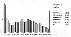
Contrast stretching by computer processing of digital data is a routine operation, although some user skill is needed in selecting specific techniques and parameters (range limits). For Landsat data, the DN range for each band, for the entire scene or a large enough subscene, is calculated and displayed as a histogram (look at the histogram for TM 3 of Morro Bay, seen earlier). Commonly, the distribution of DNs (gray levels) can be unimodal and may be Gaussian, although skewing is likely. Multimodal distributions (most frequently, bimodal but also polymodal) result if a scene contains two or more dominant classes with distinctly different (often narrow) ranges of reflectance. Upper and lower limits of brightness values typically lie within only a part (30 to 60%) of the total available range. The (few) values falling outside1 or 2 standard deviations may usually be discarded (histogram trimming) without serious loss of prime data. This trimming allows the new, narrower limits to undergo expansion to the full scale (0-255 for Landsat data). Linear expansion of DN's into this full scale is a common option.

Other stretching functions are available for special purposes. These are mostly nonlinear functions that affect the precise distribution of densities (film) or gray levels (monitor image) in different ways, so that some experimentation may be required to optimize results. Commonly used special stretches include:1) Piecewise Linear, 2) Logarithmic, Ramp Cumulative Distribution Function, 4) Probability Distribution Function, and 5) Linear with Saturation. Histogram Equalization is a stretch that favorably expands some parts of the DN range at the expense of others by dividing the histogram into classes containing equal numbers of pixels - thus, if for instance most of the radiance variation occurs over the lower range of brightness, those DN values may be selectively extended in greater proportion to higher (brighter) values.

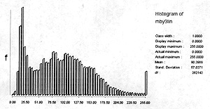
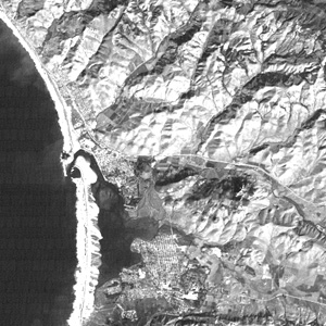
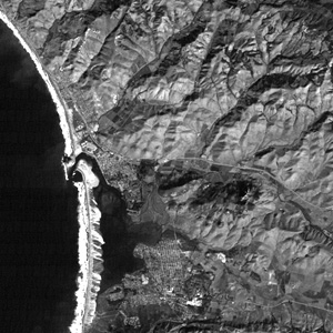
To illustrate contrast stretching (also called autoscaling) we will apply the Idrisi STRETCH function to Band 3. Recall that the histogram (see above) of raw TM values shows a narrow distribution that peaks at low DN values. One might predict from this a dark, flat image. This is indeed the case:

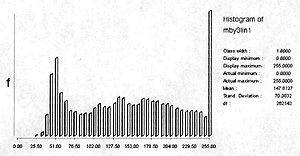
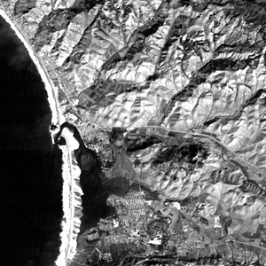
Most of the values, however, lie between DNs of 9 and 65 (there are values up to 255 in the original scene but these are few in number). We can perform a simple linear stretch so that 9 goes to 5 and 65 to 255, with all values in between stretched proportionately. This is this expanded histogram, and next to it, the resulting new image.

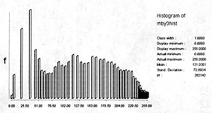
Now, most of the scene features show up as discriminable. But the image still is rather dark. Lets try instead to choose new limits in which we take DNs between 5 and 45 and expand these to 0 to 255. This results:

The histogram for this differently stretched image is polymodal, with a lower limit near 25 and a large number of DN pixels at or near 255. This accounts for the greater scene brightness (light tones).

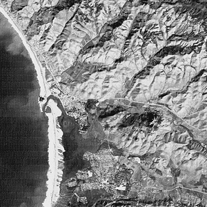
Next we try a Linear with Saturation stretch. Here we will assign the 5% of pixels at each end (tail) of the histogram to single values. The consequent histogram and image are:

The image appears as a normal and pleasing one, not much different from those we have been looking at. But comparison of this one with either of the linear stretched versions shows that real and informative differences did ensue.

Finally, we carry out a Histogram Equalization stretch, with these results:

The image is similar to the Saturation version. Note that pixel frequencies are spread apart at low DN intervals and clumped (close-spaced) together at high intervals.

Let us reiterate. Probably no other image processing procedure or function can yield as much new information or aid the eye in visual interpretation as effectively as stretching. It is the first step - and most useful function - to apply to raw data.

Another processing procedure - often divulging valuable information of a different nature - that is selectively applied, i.e., not as commonly performed, is spatial filtering. This is a technique for exploring the distribution of pixels of varying brightness over an image and, especially for detecting and sharpening boundary discontinuities. These changes in scene illumination, typically gradual rather than abrupt, produce a relation that can be expressed quantitatively as "spatial frequencies". The spatial frequency is defined as the number of cycles of change in image DN values per unit distance (e.g., 10 cycles/mm) along a particular direction in the image. An image with only one spatial frequency consists of equally spaced stripes (raster lines); for instance, a "blank" TV screen with the set turned on has horizontal stripes - this corresponds to zero frequency in the horizontal direction and a high spatial frequency in the vertical.

In general, images of practical interest consist of several dominant spatial frequencies. Fine detail in an image involves a larger number of changes per unit distance than the gross image features. The mathematical technique for separating an image into its various spatial frequency components is called Fourier Analysis. After an image is separated into its components (done as a "Fourier Transform"), it is possible to emphasize certain groups (or "bands") of frequencies relative to others and recombine the spatial frequencies into an enhanced image. Algorithms for this purpose are called "filters" because they suppress (de-emphasize) certain frequencies and pass (emphasize) others. Filters that pass high frequencies and, hence, emphasize fine detail and edges, are called highpass filters. Lowpass filters, which suppress high frequencies, are useful in smoothing an image, and may reduce or eliminate "salt and pepper" noise.

Convolution filtering is a common mathematical method of implementing spatial filters. In this, each pixel value is replaced by the average over a square area centered on that pixel. Square sizes typically are 3 x 3, 5 x 5, or 9 x 9 pixels but other values are acceptable. As applied in lowpass filtering, this tends to reduce deviations from local averages and thus will smooth the image. The difference between the input image and the lowpass image is the highpass filtered output. Generally, spatially filtered images must be contrast stretched to utilize the full range of image display. Nevertheless, filtered images tend to appear flat.

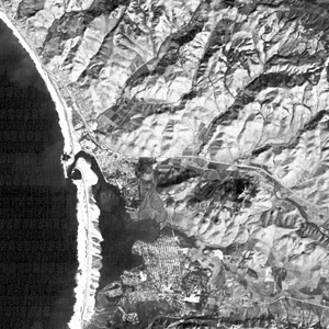
We will apply three types of filters to TM Band 2 from Morro Bay. The first displayed is a lowpass (mean) filter product, which tends to generalize the image:

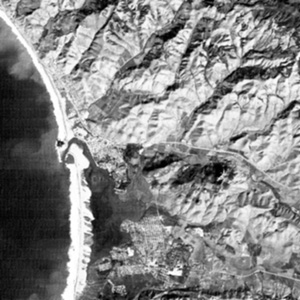
An edge enhancement filter highlights abrupt discontinuities, such as rock joints and faults, field boundaries, and street patterns:

In this example, the scene retains its general appearance but streets are singled out and some ridges are better defined. Note, too, the sediment boundaries are easier to see.

The highpass filter image for Morro Bay also brings out boundaries:

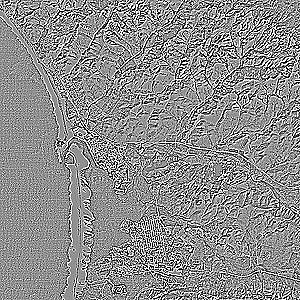
Here, streets and highways, and some streams and ridges, are greatly emphasized. The trademark of a highpass filter image is that linear features commonly are defined as bright lines with a dark border. Details in the water are largely lost. Much of the image is flat.

---

[an error occurred while processing this directive] [an error occurred while processing this directive]