Scanners like those on the Landsats (MSS; TM) were the prime earth observing sensors during the 1970s into the 1980s. But these instruments contained moving parts such as oscillating mirrors that were subject to wear and failure (although remarkably the MSS on Landsat 5 continues to operate into 1998 after launch in March of 1984). Another approach to sensing radiation was developed in the interim, namely the Pushbroom Scanner, which utilizes CCDs (Charge-Coupled Devices) as the detector. A CCD is an extremely small silicon chip which is light-sensitive. Electronic charges are developed on a CCD whose magnitudes are proportional to the intensity of impinging radiation during an instantaneous time interval (exposure time). A line of these chips is arranged in one- or two-dimensional arrays to form Solid State Video Cameras. From 3000 to more than 10000 detector elements (the CCDs) can occupy linear space less than 15 cm in length; the number of elements per unit length determine the spatial resolution of the camera. Using integrated circuits each linear array is sampled very rapidly in sequence, producing a signal that varies with the variations in radiation striking the array simultaneously. This changing signal, after transmission and recording, is used to drive an electro-optical device to make a black and white image much as is done with MSS or TM signals. After sampling, the array is electronically discharged fast enough to allow the next incoming radiation to be detected independently. A linear (one-dimensional) array acting as the detecting sensor advances with the orbital motion of the spacecraft, giving rise to successive lines of image data (analogous to the forward sweep of a pushbroom). Using filters to select wavelength intervals, each associated with its CCD array, multiband sensing is achieved. The one disadvantage of current CCD systems is their limitation to visible and near IR (VNIR) intervals of the EM spectrum.

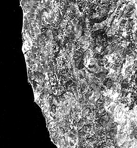
CCD detectors are now in common use on air- and space-borne sensors (including the Hubble Space Telescope which captures astronomical scenes on a two-dimensional array, i.e., parallel rows of detectors). Their first use on earth-observing spacecraft was on the French SPOT-1 launched in 1986. (The SPOT system is described in Section 3.) An example of a SPOT image, from its HRV camera, covering a 60 km section (at 20 m. spatial resolution) of the coastal region in southwest Oregon, is shown at the top. 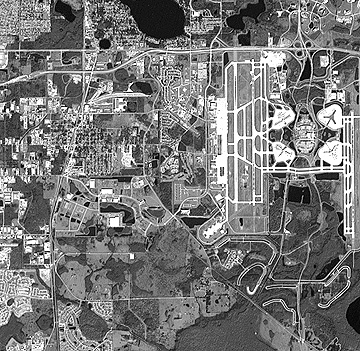Note that scan lines are absent, since each individual CCD element is, in effect, a tiny area analogous to a pixel. On its bottom is a panchromatic image (10 meters) showing the edge of Orlando, Florida, including its airport.

India has successfully operated several earth resources satellites that gather data in the Visible and Near IR, beginning with IRS-1A in March of 1988. The latest in the series, IRS-1D, was launched on September 29, 1997. Its LISS sensor captures radiation in blue-green, green, red, and near IR bands at 23 m spatial resolution. The spacecraft also produces 5.8 m panchromatic images, as well as 188 m resolution wide-field (large area) multispectral imagery. 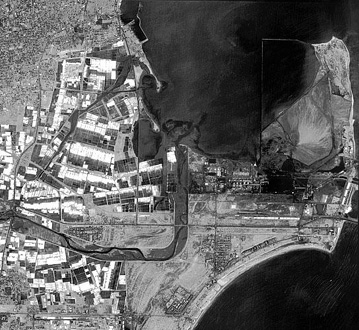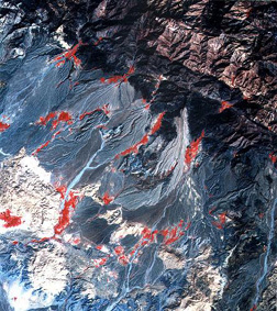Below are two recent images from this system, the one on the bottom (or right) being a 3-band color composite showing mountainous terrain and pediments with alluvium fans in southern Iran and on the top, a 5 meter panchromatic view of part of the harbor at Tamil Nadu in India:

More information on the Indian remote sensing program can be retrieved from its U.S. distributor, SpaceImaging-Eosat Corp (http://www.spaceimaging.com).

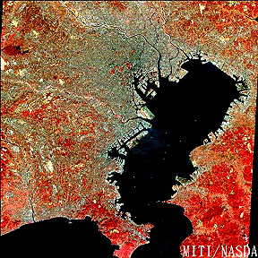
The Japanese, beginning in 1990, have flown JERS-1 and JERS-2 which include both optical and radar sensors. The optical system is a 7 band scanner similar in coverage to TM. Here is a false color image of Tokyo and Tokyo Bay:

Another major advance now coming into its own as a powerful and versatile means for continuous sampling of broad intervals of the spectrum is that of hyperspectral imaging. Heretofore, because of the high speeds of air and space vehicle movement, insufficient time is available for a spectrometer to dwell on a small surface or atmospheric target. Thus, data are necessarily acquired for broad bands in which spectral radiation is integrated within the sampled areas to encompass ranges such as, for instance Landsat, an interval of 0.1 µm. In hyperspectral data, that interval is narrowed to 10 nanometers (1 micrometer [µm] contains 1000 nanometers [1 nm = 10^-9m]). Thus, the interval between 0.38 and 2.55 µm can be subdivided into 217 units, each approximately 10 nanometers in width - these are, in effect, narrow bands. The detectors for VNIR intervals are silicon microchips; those for the SWIR (Short Wave InfraRed, between 1.0 and 2.5 µm) intervals consist of an Indium-Antimony (In-Sb) alloy. If a radiance value is obtained for each such unit, and then plotted as intensity versus wavelength, the result is a sufficient number of points through which a meaningful spectral curve can be drawn.

The Jet Propulsion Lab (JPL) has produced two hyperspectral sensors, one known as AIS (Airborne Imaging Spectrometer) first flown in 1982, the other as AVIRIS (Airborne Visible/InfraRed Imaging Spectrometer) which continues to operate since 1987. AVIRIS consists of four spectrometers with a total of 224 individual CCD detectors (channels), each with a spectral resolution of 10 nanometers and a spatial resolution of 20 meters. Dispersion of the spectrum against this detector array is accomplished with a diffraction grating. The interval covered reaches from 380 to 2500 nanometers (about the same broad interval covered by the Landsat TM with just seven bands). An image is built up, pushbroom-like, by a succession of lines, each containing 664 pixels/line. From a high altitude aircraft platform such as NASA's ER-2 (a modified U-2), a typical swath width is 11 km.

From the data acquired, a spectral curve can be calculated for any pixel or for a group of pixels that may correspond to some extended ground feature. Depending on the size of a feature or class, the resulting plot will be either a definitive curve for a "pure" feature or a composite curve containing contributions from the several features present (the "mixed pixel" effect discussed in Section 13). In principle, the variations in intensity for any 10 nm interval in the array extended along the flight line can be depicted in gray levels to construct an image; in practice, to obtain strong enough signals, data from several adjacent intervals are combined. Some of these ideas are elaborated in the block drawing shown here:

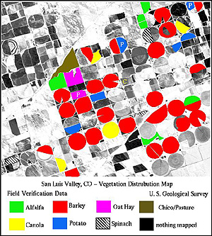
Below is a hyperspectral image of some circular fields (see Section 3) in the San Juan Valley of Colorado. Those that are colored have been identified as to vegetation or crop type as determined from ground data and from the spectral curves plotted beneath the image for the crops indicated (these curves were not obtained with a field spectrometer but from the AVIRIS data directly).

Other AVIRIS images, used for mineral exploration in the Cuprite, Nevada locality, are displayed in Section 13 (p. 13-5).

It should be obvious that hyperspectral data are usually superior for most purposes to broader band multispectral data, simply because so much more detail for the features to be identified is acquired. In essence, spectral signatures rather than band histograms are the result. Plans are in the offing to fly hyperspectral sensors on future spacecraft (see Section 20). The U.S. Navy is presently developing a more sophisticated sensor called HRST and industry is also designing and building hyperspectral instruments such as ESSI's Probe 1.

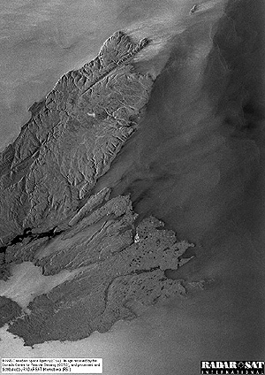
Another class of satellite remote sensors now being flown in space are radar systems (these will be treated in detail in Section 8). Among systems now operational are the Canadian Radarsat, ERS-1 and ERS-2 managed by the European Space Agency, and JERS-1 and JERS-2 under the aegis of NASDA, the National Space Development Agency of Japan. As an example, here is the first image acquired by Radarsat, showing part of Cape Breton in Nova Scotia, and surrounding waters:

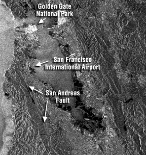
ESA, the European Space Agency, also has flown radar on its ERS-1 and ERS-2 satellites. Here is an image in black and white showing the San Francisco metropolitan area and the peninsula to its south, as well as Oakland, Calif. and the East Bay and beyond.

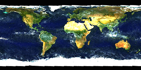
The last introductory image, also constructed from a satellite sensor that contains multispectral channels whose output is capable of being formatted into color imagery, here consists of a natural color "portrait" of the entire globe in which vegetation-rich areas are in green, vegetation-poor (including deserts) areas are in various shades of yellow and brown, and ice is displayed in white. The sensor making this composite is SeaWifs, an ocean water color satellite launched on August 1, 1997. See the oceanography subsection in Section 14 for more details of this program.

Most of the Landsat images appearing in the 20 sections of this Tutorial are individual TM bands or color composites made from diverse combinations of three TM bands, along with some MSS images. Also appearing are selected images acquired by SPOT and images made from radar and thermal sensors flown on satellites and Space Shuttle missions. A principal source for Landsat imagery and much of the astronaut space photography is the EROS Data Center (EDC) in Sioux Falls, S.D., operated by the U.S. Geological Survey. Where appropriate or necessary, principles underlying the operation of those sensors will be incorporated in the text accompanying these sections.

The U.S.G.S's EROS Data Center has assembled an Internet on-line collection of satellite images (mainly Landsat) designed to introduce the general viewer to scenes worldwide that focus on several environmental themes (e.g., cities, deserts, forests). We have linked their three page Index for this Earthshot collection which you can bring up here. To further stimulate your interest in the practicality of this imagery, in addition to its beauty, we suggest you take some time off your systematic journey through this Tutorial and sample at least those scenes that appear to be intriguing. Read through the accompanying descriptions. You may wish to return from time to time to this collection for repeat looks or to examine new examples.

We also want to introduce you to some of the computer-based processing techniques that are employed to extract information from space imagery. The main elements of such image processing are reviewed in the extended analysis in Section 1 of the first data set to be considered - a Landsat image subscene that is centered on the oceanside town of Morro Bay in California. For that, and other images in the Sections 2 and 5, we apply the Idrisi Program modules developed in part as a training tool for image processing and GIS (Geographic Information Systems) by the Geography Department at Clark University (to learn more about their system, contact them on Email at: Idrisi@vax.clark.edu. However, the capstone of this attempt to give you, the user, real familiarity with image processing techniques is reserved for Appendix 1, in which you will be taught to use PIT (PhotoInterpretation Toolkit), an interactive processing software package. Working with a training image, you will be walked through many of the processing routines, ending in your opportunity to actually classify images into thematic maps. Before trying your hand at these procedures, we suggest you wait until you complete Section 1, and perhaps the next several sections that follow it.

References on this page to foreign (non-U.S.) remote sensing systems now in operation and to U.S. distribution centers such as EROS and SpaceImaging-Eosat should clue you in to a fact now dominant in the late 1990's: remote sensing is now truly a worldwide operation. The big trend in this decade into the next century is the commercialization of space. Remote sensing is becoming a multi-billion dollar industry and new national organizations and private companies are springing forth each year to take advantage of the income-producing aspects of remote sensing as many applications (some covered in this Tutorial) of great practical value are identified. There is even a monthly magazine, EOM, dedicated to these increasing uses (http://www.eomonline.com). We shall more fully touch upon trends and issues in commercialization of remote sensing as we review the outlook for the future of remote sensing in Section 20. In that Section will also be a quick look at NASA's Regional Applications Center Program being developed by the Applied Information Sciences Branch (sponsor of this Tutorial) at NASA-Goddard.

With this Introduction into basic principles and to characteristics of Landsat and other systems behind you - and, hopefully, digested and understood - we now invite you to move on to Section 1, with its protracted tutorial development of the "whys" and "hows" of image processing, which should give you real insight and practice in(to) the efficacies of remote sensing from satellites and other types of air and space platforms.

---

[an error occurred while processing this directive] [an error occurred while processing this directive]