At each detector, the incoming light (photons) from the target knocks electrons loose in numbers proportional to the number of photons striking the detector; these electrons are removed as a continuous current passed through a counting system which measures the quantity released (radiation intensity) during each 9 microsecond detection interval; over that interval the advancing mirror picks up light coming from a lateral ground distance of 79 m (259 ft). The detector thus images a two-dimensional IFOV (instantaneous field of view, usually expressed in steradians, which denotes the solid angle that subtends a spherical surface and, in scanning, connotes the tiny area [within the total area being scanned] viewed at any one instant) of 0.087 mrad , which at Landsat's orbital altitude of 918 km determines the effective resolution of the instrument to be the 79 x 79 m² quoted above. Each detector is then cleared of its charge to receive the next 9 microsecond batch of electrons, and so on through the full forward sweep. This succession of analog signals is converted onboard into digitized values which are telemetered (sent) to Earth by radio.

For each band detector, the electronic signal from this IFOV results in a single digital value (called its DN or digital number, which for the MSS can range from 0 - 255 [2⁸]). The value is related to the proportionally averaged reflectances from all materials within the each IFOV and, since the mix of objects on the ground will constantly change, will vary in DN magnitude from one to the next IFOV. Each IFOV is represented in any b & w image of which it is a part as a tiny point of uniform gray-level tone known as a pixel (a contraction of "picture element") whose brightness is determined by its actual DN value. In a Landsat MSS band image, owing to a sampling rate effect in which there is some overlap between successive 9 microsecond intervals, a pixel has an effective ground-equivalent dimension of 79 by 57 m (259 x 187 ft) but contains the reflectances of the full 79 m² actually viewed .The average (but variable) number of pixels within a full scan line (representing 185 km) across the orbital track is 3240 (185 / 0.057). In order to image an equi-dimensional scene, which requires 185 km of down track coverage, the average total number of lines to do this is set at 2340 (185 / 0.079). Each band image will therefore consist of approximately (again variable) 7,581,600 pixels - a lot to handle during computer processing.

The continuous stream of pixel values can be used to drive an electronic device that generates a uninterrupted light beam of varying intensity which sweeps systematically over film to produce a b & w photo image in which tone variations are proportional to the DNs in the array. Or, the pixels generated from these sampling intervals can be displayed as an image of each band by feeding their DN values sequentially into an electronic signal array. That is then projected line by line on to a TV monitor (in which the resulting image is an assemblage of light-sensitive spots [also called pixels] of varying brightnesses).

We now introduce you to your first Landsat image, an October 1972 scene.On your screen is displayed a succession of MSS bands 4 through 7 (bands 1-3 were assigned to the RBV) comprising images that cover a very well known region in the eastern U.S. Below these is a false color composite, made from bands 4, 5, and 7, of this scene, here extended southward to include the southern tip of a peninsula that includes the town of Cape May (clue). Before scrolling on, make an educated guess as to what geographic area is shown here. Try your hand at picking out major landmarks in the scene (use an atlas for help in recognizing their locations).

(Note 1: By convention Landsat [and most other satellite system] images are normally oriented with North towards the top; however, because of the 9 degree orbital inclination, the north direction is not vertical but is a few degrees inclined relative to the perpendicular to the top and bottom margins of the printed image.) (Note 2: The lettering at the bottom of each image [probably not readable on your screen] is the standard annotation placed on Landsat images produced at NASA, EROS, and most commercial facilities; the information recorded, from left to right, includes the calendar date of acquisition, the latitude-longitude coordinates of the scene principal and nadir points, the sensor type, the elevation and azimuth positions of the Sun, and the Scene [Frame] identification number [I.D.] starting with the particular Landsat (1 through 5) and ending with the specific band [or band combination if in color].)

Landsat MSS October 10, 1972

	MSS Band 4
	MSS Band 5
	MSS Band 6
	MSS Band 7
	MSS Band 4 = Blue MSS Band 5 = Green MSS Band 7 = Red

You probably arrived at the correct scene identification: In the individual bands, much of New Jersey is shown along with New York City and the west end of Long Island in the upper right corner and Philadelphia at bottom left center. The color composite extends the coverage to include the northern Delmarva Peninsula flanked by the northern Chesapeake Bay (left) and Delaware Bay (center) and Cape May. These two urban regions, along with Trenton on the Delaware River and the New Jersey cities along the Hudson appear in light to medium gray tones in Band 5 (red). In Band 7 (IR), the central areas of these metropolitan complexes are rendered in dark tones, owing largely to the prevalence of asphalt streets and dark (usually asphalt) roofs together with low concentrations of trees and other vegetation, an effect enhanced by the contrast to light tones associated with vegetation in the countryside. Water is dark in Bands 6 and 7 but lighter in Bands 4 and 5 in part because of silt and other sediments (more reflective). In contrast, among the brightest features in both individual band and color composite scenes are the sandy beachs and soils making up the ocean side of the barrier islands lining the Jersey coast. Vegetation in this October 10. 1972 scene is still actively growing (mostly green; some trees are beginning to get their autumn colors), so its distribution is indicated by the overall brightness in the Band 6 and 7 images (contrast the dark tones of the fold belt ridges in the upper left in Band 5 with their corresponding light tones in Band 7). The large, darker area in New Jersey east of Philadelphia is the Pine Barrens, marked by evergreens that grow well in the sandy soils there (note its appearance also in each of the four bands).. Surfaces dominated by vegetation are shown in several shades of red in the false color composite. Harvested (fallow) fields appear in blue tones, similar to those characterizing the cities.

As a preview of what is known as change detection, compare the October Band 7 image with the one shown below which was taken on April 18, 1978, a time in the Spring in which trees and other vegetation have not yet leafed out (note the especially dark ridges whose tones result from rock and soil reflectances). Many of the bright areas in this April image do correlate with some field crops that were planted earlier; small bright patches in the Pine Barrens are sand pits - highly reflective in all bands.

The MSS is capable of simulating rather crude spectral signatures. Bands 4, 5, and 6 each have a bandwidth of 0.1 mm; band 7's width is 0.3 mm. Band responses can be represented by bars in a histogram-like plot in which the height of the bar signifies the relative reflectances averaged for all wavelengths within the bandwidth interval. This we show here with an illustration from the U.S. West Coast:

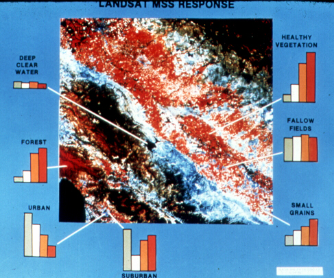
The scene is the first color composite made from ERTS-1 digital data. This includes Monterey Bay (lower left), the Coast Ranges below San Francisco, the Sacramento (Great) Valley, and the western slopes of the Sierra Nevada. Notice that the pattern of each histogram set, for a particular surface cover type, differs from the others. Thus, each class of material has a distinctive signature, approximated by the 4 bars, that sets it apart from the others. To simplify, the width of band 7 (bar on the right) is made equal to the other three. Urban is most reflective in Bands 4 and 5; suburban is strong in Bands 4 and 7 (the latter tied to the influence of planted vegetation). The signatures for forest and healthy croplands are similar but the heights of the bars for Bands 6 and 7 are greater for the crops; the bar heights for small grains and fallow fields are similar but the response for Bands 4 and 5 is just a bit higher than for 6 and 7. The two very dark areas in the Coast Range and in the Sierra Nevada (not shown as histograms) result from the predominance of conifers.

Next, refer to the table that will come up on the next screen in which some criteria are presented for using combinations of band gray tones or colors and their patterns to identify land cover categories. Again, apply these to see if you can recognize examples of any such categories in this scene. Become familiar with this table as we will challenge you to practice this approach whenever you examine various Landsat scenes (and imagery from some of the other earth-observing satellites) in this Tutorial.

---

[an error occurred while processing this directive] [an error occurred while processing this directive]